Current World Environment

Introduction

Coastal shrimp aquaculture in a traditional form existed in Indian sub-continent for many centuries. During eighties the shrimp farming enterprise picked momentum and became a popular farming practice among coastal farmers. It was in the 1990 s, the economic liberalization process widened the scope of the commercial shrimp farming since it was arose an export oriented  activity. The government schemes and programmes fueled the growth in subsequent years and the shrimp farming become a very important sub-sector of the fisheries domain. During the year 2013-14, India exported shrimp worth Rs 19368 crores(MPEDA,2014).Shrimp farming is dependent on various factors like quality of the physical characteristics of the system, climatic conditions and essentially the quality of all the input resources that are used in the production process. Hence,theshrimp yield is a function of  different factors. The variation in the yield and the factors responsible for the inefficiencies has to be studied in detail to improve the production and productivity of the farms and thus our farming systems can achieve maximum efficiency.

Materials and Methods

In this study we have collected farm level cross sectional data from randomly selected 150 shrimp farmers of East Godavari district. A interview schedule was pretested and used to collect the information from the farmers. Stochastic production function was used to explain the variation in the shrimp yield.The stochastic frontier model has been widely used in  measurement of performance of agriculture in developing countries where the data are often  influenced by measurement errors and other stochastic factors such as weather conditions, diseases, etc (Aigner et al, 1977). The Technical Efficiency (TE) estimation has also been attempted by many researchers in aquaculture economics, majority of those studies are from Asian countries. (Shang et al. 1998;Sharma et al.1999; Iinuma et al. 1999; Sharma and Leung 2000; Irz and McKenzie 2003; Chiang et al. 2004; Dey et al. 2005; Singh et al. 2009; Alam et al. 2011; Rahman et al. 2011;). To estimate the Technical Efficiency the Battese and Coelli (1995) model is widely adopted model due to its computational simplicity and ability to examine the effects of various farm specific variables of TEin an econometrically consistent manner. This model was employed in recent studies.Sharma and Leung (2000); Dey et al. (2000, 2005) ; Singh et al. (2009); Alam et al. (2011) have employed the FRONTIER 4.1 software, used Battese and  Coelli (1995), to  simultaneously estimate the parameters of the SPF and the TE models. The stochastic frontier production function for cross-sectional data is specified as: Y_i=f (X_i; β)  exp (V_i − U_i )(1) Where Y_i denotes the production for the i th farm (i = 1, 2, 3,  ... ... ., n ), X_iis a 1 × k  vector of the value of known functions of inputs of farm production and of other explanatory variables associated with the i th farm, β is a k × 1 vector of unknown parameters to be estimated, V_i’s are random variables which are assumed to be independently and identically distributed N (0, σ_v²) and independent of the U_i’s,U_i’s are non-negative random variables associated with TE in  production and are  assumed  to  be  independently  distributed as truncations of the N (Z_iδ, σ_u²) distribution. Following Battese and Coelli (1995), U_i’s can be represented as: U_i=Z_iδ + W_i(2) where Z_i is a 1 × p vector of variables which may  influence  efficiency  of  a  farm,  δ  is  a p × 1  vector  of  parameters  to  be  estimated, W_i’s  are random  variables  defined by  the  truncation  of  the  normal  distribution with mean 0 and variance σ_u² , such that the point of truncation is −Z_iδ, that is, W_i≥ Z_iδ. These assumptions are consistent with U_i being a non-negative truncation of the N (Z_iδ, σ_u²) distribution (Battese and Coelli, 1995). By using the maximum likelihood (ML) estimation procedure simultaneous estimation of the parameters of the stochastic frontier model is possible as in Eq. (1) and those for the technical inefficiency model in Eq. (2) the likelihood function and its partial derivatives with respect to the parameters of the model are given.(Battese and Coelli,1993). The technical efficiency of production for the i th farm (TE_i) is defined as:

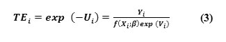
Given the model assumptions, the prediction of the TE’s is based on the conditional expectation of the expression in (3).  

Empirical Model

The  stochastic production frontier for shrimp farming in Andhra Pradesh can be estimated using the  Cobb–Douglas  functional  form  as specified below:

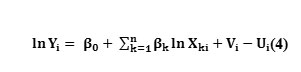
where subscript i refer to the ith farm in the sample; ln represents the natural logarithm; Y represents output and X’s are input variables defined earlier; δ’s are parameters to be estimated; V ’s and U’s are random variables defined earlier. Maximum likelihood estimation of Eq. 4 provides the estimations for b’s and variance parameters,

Following Battese and Coelli (1995), it is assumed that the technical inefficiency distribution parameter, U_i is a function of various operational and farm-specific variables hypothesized to influence technical inefficiencies as:

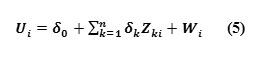
Where Z’s are various operational and farm-specific variables, defined earlier;’s unknown parameters to be estimated; and W_i’s are also defined earlier. It should be noted that the technical inefficiency model in Eq. 5 can only be estimated if the technical inefficiency effects, U_i’s, are stochastic and have particular distributional properties Coelli and Battese, (1996). Therefore, it is of interest to test the null hypothesis for the absene of technical inefficiency effects,ϒ = δ₀= δ₁ =.....=δ₉ = 0; that technical inefficiency effects are nonstochastic, ϒ = 0 and that farm-specific factors do not influence the inefficiencies, δ₁ =.....=δ₉ Ounder ϒ= 0; the stochastic frontier model reduces to a traditional average function in which the explanatory variables in the technical inefficiency model are accounted in the production function. These hypothesis and related null hypotheses can be tested using the generalized likelihood-ratio statistic λ given by:


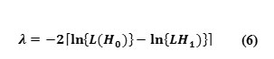
Where L(H) and L(H₁) denote the values of likelihood function under the null and alternative (H₁) hypotheses, respectively. If the given null hypothesis is true, λ has approximately X²  distribution or mixed X² distribution when the null hypothesis involves y = 0. Given the model specifications, the Technical Efficiency  index for the i^th farm in the sample TE_i , defined as the ratio of observed output to the corresponding frontier output, is given by: TE_i = exp (-U_i)  (7) The prediction of TE is based on the conditional expectation of expression in Eq. (7) given the values of V_i - U_i evaluated at the maximum likelihood estimates of the parameters of the stochastic frontier model (Battese and Coelli, 1988). The frontier production for the i^th farm can be computed as the actual production divided by the TE estimate. The parameters for the stochastic frontier function in Eq.  (4)  and those  of  the  technical  inefficiency model  in Eq. (5) are estimated simultaneously using the ML estimation method, using the computer program, FRONTIER 4.1 (Coelli, 1994).

Output and Input Variables

The variables corresponding to the output and input parameters involved in the stochastic production frontier function for the sample shrimp farmers in  East Godavari district, Andhra Pradesh are given in Table 1.  Water spread area, stocking density, quantity of feed, labour cost, cost of chemicals and fertilizers, cost of electricity and fuel   are included in the SPF. The efficiency of farm might be affected by the farm specific variables that are mentioned in the Table 1. Based on the existing literature, the variables were chosen and the justification for their inclusion also elaborated.

Table 1: Specification of Variables in the Stochastic Production Frontier and Technical Inefficiency
Model for Shrimp Farming.

Variable	Description	Unit
Y	Total shrimp production  per hectare per year	kg
Variables in the production frontier
X Ws	Water spread Area	Ha
X Pl	Quantity of  post larvae stockedper hectare per year	Number
X Fd	Quantity of feed used per hectare per year	kg
X La	Labour cost per ha	Rs /ha
X Cf	Cost of chemicals and fertilizers applied per hectare per year	Rs /ha
X Cf&e	Cost of fuel and electricity consumed per hectare per year	Rs /ha
Variables in the inefficiency function
Z Cd	Culture Duration	Days
Z Ag	Age of the shrimp farmers	Yrs
Z Ex	Experience of the shrimp farmers	Yrs
Z Ed	Education level of the shrimp farmers(Primary 1, Secondary 2 , Higher Education 3)	yrs
Z Oc	Shrimp farming as primary occupation  (1 if yes , otherwise 0)	1, 0
Z Fa	Family size of the shrimp farmers	Persons
Z Rk	Risk Averse nature of the shrimp farmers (1 if yes, 0 otherwise)	0,1
Z Ea	Early technology adoption nature of the shrimp farmers (1 if yes, 0 otherwise)	0,1
Z Ls	Farm ownership (if leased then 1, otherwise 0)	1, 0
Z Me	Membership in shrimp Farmers Associations  and societies (1 if yes, 0 otherwise)	1,0

 
Results and Discussion Farm Characteristics

Characteristics of the sample shrimp farms were presented in the Table 1. The average water spread area of the farms was found to be 1.06 ha. The farms stock an average of  Rs391502 PL per ha that is equivalent to 39 PL per square meter. Shrimp were fed with  commercial pellet feed, the average quantity of feed applied was Rs11251 kgs. The mean shrimp production ranged from Rs 3128 kg/ha to Rs 11326 kg/ha and the average production was Rs 7846 kg/ha. The amount of labour used for  production was expressed in terms of salaries and wages paid for  permanent labour as well as hired labour utilized for specific activities such as pond preparation and other regular activities . The average labour cost is Rs 51135/ha. Farmers use a variety of chemicals and fertilizers right from the stage of pond preparation to the harvest. The average cost of chemicals and fertilizers is Rs189507/ha. The average cost of electricity and fuel is Rs 245036 /ha.

Table 2 Summary Statistics of the Variables Involved – East Godavari District.

Name of the variable	Minimum	Maximum	Mean	Std Dev
Shrimp Yield (kg/ha)	3128	11326	7846	1826
Water Spread Area (ha)	0.45	1.6	1.06	0.27
Stocking Numbers (No/ha)	150000	550000	391502	98436
Feed (kg/ha)	4461	16343	11251	2462
Labour cost (Rs/ha)	19358	65987	51135	10265
Cost of Chemicals & Fertilizers (Rs/ha)	69194	26832	189507	44126
Cost of Electricity and Fuel (Rs/ha)	91410	407545	245036	60923
Duration of Culture (Days)	62	131	106.77	13.97
Age (Years)	29	65	44.21	8.56
Education (1 or 2 or 3)	1	3	1.87	0.63
Experience (Years)	7	25	13.13	4.62
Family size (No)	2	6	3.52	1.19
Occupation (0 or 1)	0	1	0.78	0.42
Ownership (0 or 1)	0	1	0.69	0.46
Membership (0 or 1)	0	1	0.55	0.5
Risk averse (0 or 1)	0	1	0.46	0.5
Early-adopt (0 or 1)	0	1	0.62	0.49

Parameter Estimates of the Inefficiency Function

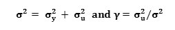
In TE analysis, the dependent variable of the inefficiency model in Eq. (5) is defined in terms of the level of inefficiency; a farm-specific variable associated with the negative (positive) coefficient will impact  positively (negative) on TE. From the results it is observed that experience and educational status of the farmers has significant positive effect on the TE of the farm. Age was found to be positively associated with the TE. These results suggest that farmers with higher experience and better education were taking proper farm management decisions which increased their TE. These results were also supported by the studies carried out by Dey et al. (2000), Alam et al. (2011), and Rahman et al. (2011). A part from these variables early technology adopting nature, and membership with organizations were also found to be positively related with the TE. These variables were associated with the TE at 5 % significant level, whereas risk averse nature, family size, occupational status and ownership status were negatively associated with TE. Though  family size, occupational status, duration of culture, ownership status were negatively related, the statistical significance was only at 10% level. The estimated γ parameter associated with the variance in the stochastic production frontier model is found to be close to one and highly significant. Though the γ parameter cannot be interpreted as the proportion of the total variance explained by the Technical Efficiency effects, from the result it is inferred that Technical Efficiency effects do have a significant contribution to the variation of shrimp production in Andhra Pradesh.

Technical Efficiencies

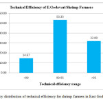Figure 1: Frequency distribution of technical efficiency for shrimp farmers in East Godavari District Click here to View figure

Fig.1 depicts the frequency distribution of the estimated TE scores for the sample shrimp farmers in East Godavari district. About 32 % of farmers have TE scores above 95%, while 53.33 % operate between 90 and 95%. About 14.67 % farmers operate at less than 90%. The mean TE level of shrimp farmers was found to be 93.06 %. Similar kinds of results were obtained by Reddy et al (2008) in a study in East Godavari district, where the estimated TE of shrimp farming was 93%. Studies conducted in other countries had lesser TE scores. For example, studies conducted in Bangladesh shrimp farming systems shows that the Technical Efficiency scores were found to be around 70 %. Haque (2011) found the Technical Efficiency of shrimp culture to be 71%.  Rahman et al (2011) concluded that the Technical Efficiency of shrimp culture at 68%.

Conclusions

From the study it is clearly evident that farmers were technically efficient and they could achieve 93.06 % of the potential yield in East Godavari. The reason for the higher TE was probably due to the better understanding of the production technology by the farmers.  The semi intensive farming technology the farmers adopt is a superior production technology in which high quality commercial pellet feed is used to feed the shrimps and a variety of growth enhancers are also applied to the pond ecosystem during different stages of the growth cycle. The gap in the TE scores indirectly informs that  there is still good scope to improve their production to achieve the potential yield. The main factors that contribute to the inefficiency were experience, education and age of the farmers. The early technology adopting nature and membership with organizations were positively related with the TE. Family size, occupational status, duration of culture, ownership status was negatively related with TE. The study results imply that the gap in TE maybe attributed to the farmers’ personality traits. Valderrama et al (2014) suggests that the efficiency of the farms can be improved with proper technical training programs to farmer son Better Management Practices that will enable them to achieve better productivity further.

References
 

1. Aigner,D.,Lovell,C.A.K.and Schmidt,(1977).Formulation and Estimation of Stochastic Frontier Production Function Models.Journal of Econom
2. Alam,M.F.aMurshed-e-Jahan.,2008,‘Resource allocation efficiency of the prawncarp farmers of Bangladesh’,Aquaculture Economics & Management,12(3), pp.188-206
3. AlamMFerdous,Md.Akhtar uzzaman Khan,A. S.M. AnwarulHuq2011,‘Technical efficiency in tilapia farming of Bangladesh:as to chastic frontier production approach’,Springer Science and Business
4. Batese,G.E. and Coelli,T.J.(1995).AModel forTechnical Inefficiency Effectsina Stochastic Frontier Production Function for Panel Data. Empirical Econom
5. Binam,J.N. (2004). Factors Affecting the Technical Efficiency among Small holder Farmers in the Slash and Burn Agriculture Zone of Cam
6. BuiLeThaiHanh,(2008).Impact of Financial variable son the production efficiency of Pangasius farms in An Giang province, Vietnam.
7. Chiang, F., Sun, C. and Yu, J. (2004). Technical efficiency analysis of milk fish (Chanos chanos) production in Taiwan - an application of the stochastic frontier production function.
8. Coelli, T. J. 1994. A guide to FRONTIER version 4.1: a computer program for stochastic frontier production and cost function estimation. Department of Econometrics, University of New England, Armidale, Australia.
9. Coelli,T.,Prasada Rao,D.S. and Batese,G.E.(1998).An Introduction to Efficiency and Productivity Analysis,Kluwer Academic Publishers, Bo
10. Coelli, T.J. (1996). “A 1: A ComputerProgram for Stochastic Frontier Production and Cost Function Estimation”, CEPA Working Paper 96/7, Department of Econometrics, University of New England, Armidale NSW Australia.
11. Coelli, T. J. and G. E. Battese. 1996. Identification of factors which influence the technical efficiency of Indian farmers. Austrian Journal of Agricultural Economics 40(2):103–128.
12. Debreu, Koopmans, (1951) and Farrell, (1957). Stochastic non-parametric frontier analysis in measuring technical efficiency: a case study of the North American dairy industry.
13. Den, D. T., T. Ancev, et al. 2007, ‘Technical Efficiency of Prawn Farms in the Mekong Delta, Vietnam’, Australian  Agricultural  and  Resource  Economics  Society,  New Zeal and
14. Dey,M., Paraguas,F.J.,Bimbao,G.B. and Regaspi,P.B.(2000).Technical Efficiency of Tilapia Grow out Pond Operations in the Philippines. Aquaculture Economics and Management.
15. Dey, M. M., F. J. Paraguas, et al. 2005, ‘Technical efficiency of freshwater pond poly-culture production in selected Asian countries: estimation and   implication’, Aquaculture Economics & Management, vol. 9(1-2): 39-63
16. Farrell, M. J. 1957, ‘The Measurement of Productive Efficiency’, Royal Statistical Society,120: 253-2990
17. Hanh, Bui Le Thai 2009, ‘Impact of financial variables on the production efficiency of Pangasius farms in An Giang province, Vietnam’, MSc. thesis, University of Tromsø, Norway & Nha Trang University, Vietnam.
18. Haque, S. 2011. Efficiency and institutional issues of shrimp farming in Bangladesh. Faming and rural systems economics. Margraf Publishers, Weikersheim, Germany.
19. Irz, X. and V. Mckenzie. 2003. Profitability and technical efficiency of aquaculture systems in Pampanga, Philippines. Aquaculture Economics and Management 7:195–211.
20. Iinuma, M., K. R. Sharma, et al., 1999, ‘Technical efficiency of carp pond culture in peninsula Malaysia: An application of stochastic production frontier and technical inefficiency model’, Aquaculture, vol. 175 (3-4), pp.199-213.
21. Kaliba, A. R. and C. R. Engle., 2006, ‘Productive efficiency of catfish farms in Chicot county, Arkansas’, Aquaculture Economics & Management, vol. 10(3): 223-243.
22. 2014. www.mpeda.com
23. Rahman, S., B. K. Barmon, and N. Ahmed. 2011.Diversification economics and efficiencies in a “bluegreen revolution” combination: a case study of prawn carp-rice farming in the “gher” system in Bangladesh. Aquaculture International 19:665–682.
24. Reddy, G. P., M. N. Reddy, B. S. Sontakki, and D.B. Prakash. 2008. Measuring of efficiency of shrimp (Penaeus monodon) farmers in Andhra Pradesh. Indian Journal of Agricultural Economics 63(4): 653–657.
25. Sathiadhas, R and Najmudeen, T M and Prathap, K Sangeetha 2009, ‘Break-even Analysis and Profit ability of Aquaculture Practices in India’, Asian Fisheries Science, vol. 22 (2), pp. 667-680.
26. Sivaraman I (2014~) A critical analysis of better management practices in shrimp farming in Andhra Pradesh, Fisheries Economics, Extension and Statistics Division, Central Institute of Fisheries Education, Mumbai, Unpublished Ph.D thesis (work in final stages)
27. Sharma, K.R., Leung, P., Chen, E., Peterson, A., 1999, ‘Economic efficiency and optimum stocking densities in fish poly-culture: An application of data envelopment analysis (DEA) to Chinese fish farms’, Aquaculture, 180, 207– 221
28. Sharma, K. R. and P. S. Leung 2000, ‘Technical efficiency of carp production in India: a stochastic frontier production function analysis’, Aquaculture Research, vol. 31(12): 937-947.
29. Shang, Y. C., P. Leung, and B.-H. Ling. Comparative economics of shrimp farming in Asia. Aquaculture 164(1–4):183–200.
30. Singh, K., M. M. Dey, A. G. Rabbani, P. O. Sudhakaran, and G. Thapa. 2009. Technical efficiency of freshwater aquaculture and its determinants in Tripura, India. Agricultural Economic Review 22:185–195.
31. Timothy J. Coelli, D.S. Prasada Rao, et al. 2005, ‘An introduction to Efficiency and Productivity Analysis’, Second Edition, Springer: 172.
32. Ton Nu Hai Au, (2008). Aquaculture Economics and Management; Technical efficiency of prawn poly-culture in Tam Giang lagoon, ThÆ°a Thien Hue, Vietnam
33. Tran Thanh Xuan, (2001). Survey, study and sensible application of coastal estuary eco- system of Mekong River network for resource protection and aquaculture develop m Scientific report, Research Institute for Aquaculture No2.
34. Valderrama Diego , Sivaraman Iyemperumal & M. Krishnan (2014) Building consensus for sustainable development in aquaculture: A Delphi study of better management practices for shrimp farming in India, Aquaculture Economics & Management, 18:4,369-394, DOI: 10.1080/13657305.2014.959211