Determination Discharge Capacity of Triangular Labyrinth Side Weir Using Multi-Layer Neural Network (ANN-MLP)
Sohrab Karimi1 , Hossein Bonakdari1 * and Azadeh Gholami1
http://dx.doi.org/10.12944/CWE.10.Special-Issue1.16
statistic indexes have been used to assess the accuracy of the results. The results of the examinations indicate that using MLP model along with simultaneous use of dimensionless parameters for the purposes of estimating discharge coefficient: the ratio of water behind the weir to the channel width (h/b), ratio of weir crest length to weir height (L/W), relative Froude number (F=V/√(2Side weirs are used in open channels to control flood and the flow passing through it. Discharge capacity is one of the crucial hydraulic parameters of side weirs. The aim of this study is to determine the effect of the intended dimensionless parameters on predicting the discharge coefficient of triangular labyrinth side weir. MAPE, RMSE, and Rgy)) and vertex angle (Ï´), offered the best results (MAPE= 0.67, R2= 0.99, RMSE = 0.009) in comparison with other models.
Copy the following to cite this article:
Karimi S, Bonakdari H, Gholami A. Determination Discharge Capacity of Triangular Labyrinth Side Weir Using Multi-Layer Neural Network (ANN-MLP). Special Issue of Curr World Environ 2015;10(Special Issue May 2015). DOI:http://dx.doi.org/10.12944/CWE.10.Special-Issue1.16
Copy the following to cite this URL:
Karimi S, Bonakdari H, Gholami A. Determination Discharge Capacity of Triangular Labyrinth Side Weir Using Multi-Layer Neural Network (ANN-MLP). Special Issue of Curr World Environ 2015;10(Special Issue May 2015). Available from: http://www.cwejournal.org
Download article (pdf) Citation Manager Publish History
Introduction
Side weirs are amongst hydraulic structures used for varied purposes in water transfer systems, irrigation networks, drainage, surface water collection systems, sewers and wastewater discharge ducts, and water and sewerage treatment plants. Diverting surplus discharge in rivers and channels is among other applications of side weirs. Moreover they are constantly and widely used for specific impounding of rivers or channels. The flow in the weirs is a spatially varied flow (Borghei, 2011). A spatially varied flow is a type of permanent flow in which the flow intensity increases or decreases in the channel along the flow direction. When the flow is a spatially varied flow it decreases along the path as discharge decreases, which is basically a diverted flow (DeMarchi G, 1934). Labyrinth and normal side weirs are among different types of weirs. Labyrinth weirs are constructed in a spiral manner so that they will create a larger weir crest length in comparison with the normal weirs. This increases the passing discharge in comparison to a normal weir with similar head and similar side space. Labyrinth side weirs are used as a structure to better overflow the flow in larger containers and it allows the overflow threshold to increase when the water is at its maximum level. Labyrinth weirs could be sharp- crested and broad- crested and normal weirs are built in varied shapes such as rectangle, triangle, trapezium, circle, and … (Kumar et al., 2011; Wormleaton and Tang, 2002; Emiroglu and Baylar, 2005).
DeMarchi (1934) solved the dynamic equation of discharge- decreasing spatially varied flow for the first time in 1934 for rectangular horizontal channels when the friction can be overlooked with the premise that the energy is constant along the weir. Subramanya and Awasthy (1972) studied the general differential equation of spatially varied flows with decreasing discharge in a horizontal rectangular channel and presented a number of equation for discharge coefficient for the sharp- crested side weirs through conducting a series of experiments on subcritical and supercritical flows. They also measured the velocity profiles and demonstrated that the rectangular side weir will have a significant effect on velocity distribution near the weir.
Considering the complexity of engineering problems and growing engineering studies, new methods called soft calculation were significantly used during recent decade which showed more efficient and more accurate to solve complicated and difficult engineering issues. Emiroglu et al. (2009) were able to obtain the discharge coefficient of triangular weirs through using (ANFIS) fuzzy neural network. The discharge coefficient is dependent on the geometrical parameters of the main channel and the weir in the model presented by them . Kisi et al. (2012) were able to obtain the discharge over the triangular weir through using neural network (ANN). The upstream weir Froude number, the weir length, the main channel width, the weir height, the angle of the apex of the triangular weir, and the upstream water height were the parameters affecting the discharge coefficient in their study .
Bilhan et al. (2010) succeeded in developing the neural network(ANN) method and obtaining the discharge coefficient of rectangular weirs through other neural network models. These models include: FFNN and RBNN models. Dursun et al. (2012) conducted their studies on elliptical weirs and were able to obtain an equation for discharge coefficient in such weirs. They utilized the (ANFIS) fuzzy neural network in their examinations and compared the results with that of other methods .
Multi-layer neural network (ANN-MLP) is one of the methods taken in to use in water hydraulic engineering during recent years. One of the benefits of this method which can be pointed out is the desirable performance of it in analyzing complex flows (Kisi, 2008; Bonakdari et al., 2011; Baghalian et al., 2012; Donmez, 2011; Huai et al., 2013).
The main purpose of the present study is to predict discharge coefficient through using the MLP method. The factors influencing the determination of discharge coefficient were first specified through using sensitivity analysis in order to fulfill the purpose of this study. Six models are then presented considering each of these dimensionless parameters. And then the discharge coefficient has been predicted through training and testing the MLP network for each of the presented models. RMSE, MAPE, and R2 statistical parameters were finally used to compare the six above- mentioned models. The best and most effective parameters in predicting the discharge coefficient will be introduced at the end.
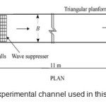
Experimental Model (Kumar et al, (2011)
Present study used Kumar et al, (2011) experimental data to estimate discharge coefficient. A horizontal rectangular channel with 12 meter length, 0.28 m width and 0.41 meter height was used in the experiments. The weir used was a triangle located 11 meter away from channel entrance. Water height over weir crest was measured by point gages having ±0.1 mm accuracy. To create edge flow over the weir, air conditioning pits were used. Network walls and wave preventers were structured to eliminate the vertex and water surface disturbance. Table 1 shows the parameters used in present study.
 |
|
Table1: Parameters used to estimate average discharge coefficient (Kumar et al, 2011)
|
h/b |
L/h |
F |
L/w |
θ (degree) |
Cd |
|
|
min |
0.260714 |
135.25 |
0.608 |
11.76087 |
30 |
0.54 |
|
max |
0.028571 |
3.888889 |
3.261 |
2.685185 |
180 |
0.906 |
Multi-Layer Neural Network
The Multi-layer neural network is considered one of the soft computing methods. One of the benefits of this method which can be pointed out is the desirable performance of it in analyzing complex flows. Also the nonlinear models of current can also be studied through this method. The basis of the process in this method is training and learning processes. The components of the structure of artificial neural network(ANN) include: hidden layers, hidden units and hidden neurons, input layer, output layer ( Yang and Chang, 2005; Smith, 1993).
The flexible structure of artificial neural network (ANN) makes it capable of modeling complex and nonlinear patterns between input and output data. The capability to estimate the accurate results is done through using input data on the basis of training and learning process. What is meant by training the neural network is to obtain the weights (w) of the network. Also classifying different types of ANN is done based on the methods of obtaining the weights and also the utilized transfer functions. One of the various types of neural network which is used frequently is Multilayer Perceptron (MLP). An MLP feed forward includes an input layer, one or more hidden layers and an output layer (Figure 2). Each layer is made up of a number of neurons the number of neurons in the input and output layers are equal to the number of inputs and outputs of the under- study issue respectively. Various types of functions could be considered as sigmoid function, hyperbolic tangent was used as activation function in the hidden layers in this study. Levenberg- Marquardt method was used for training of ANN (Melesse et al., 2011; Van Maanen et al., 2010). Back- propagation algorithm, which is one of the most beneficial algorithms, is used in this method in order to figure out the weights and bias of the neural network. This algorithm minimizes the difference between the observed outputs from the experimental studies and the ANN model outputs very quickly through determining weights and bias.
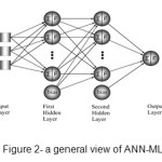 |
Fig. 2: a general view of ANN-MLP Click here to View figure |
The modeling and simulation of ANN-Multilayer Perceptron (MLP) was written by matlab programming language in this study. In order to analyze and solve a neural network which has two hidden layers and in order to determine the number of the existing neurons in each layer, trial and error method was used. The functions and equations which are analyzed for the output layer are linear, ( Bilgil and Altun, 2008; Asadi et al., 2013; Bilhan et al., 2011).
The way the trial and error method works is that various runs are taken in order to determine the number of neurons of the layers of the neural network in case the number of the neurons are not equal in the first and the second layer and then the RMSE error is determined for each of them separately and the state which has the least amount of error will be selected as the base for modeling ANN. These parameters (model 1-6) are placed in the first layer of the neural network as the input parameters. The neural network will be trained through a number of these parameters within the middle layer in the following stage so that they could gain their optimum structure and after reaching the already- determined stopping point, the training process will stop. As said earlier the purpose of the structured neural network is to estimate the discharge coefficient.
Method
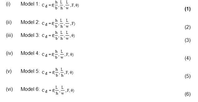
Through examining the studies conducted in the field of discharge coefficient it could generally be states that the dependent Cd parameter is dependent on the ratio of water behind the weir to the channel width (h/b), the ratio of the weir crest length to the water height behind the weir (L/h), the ratio of the weir crest height to the weir height (L/w), the approximate Froude number (F=V/√(gy)), and the vertex angle (θ) independent dimensionless parameters. Therefore the six models could be presented as below through using the presented dimensionless parameters. It could be seen that model number 1 includes all the presented dimensionless parameters and models 2 to 5 examine the effect of not considering each of the presented dimensionless parameters.
In order to verify the accuracy of the estimated model, at each step of model development, the results of analysis of MLP for each model is based on the criteria of coefficient of determination (R2), Root Mean Square Error (RMSE), Mean Absolute Percentage Error (MAPE), as defined in the following forms.
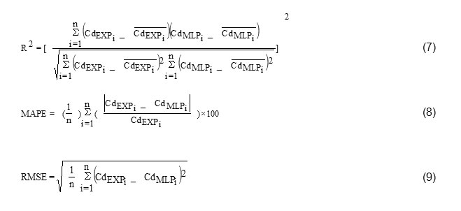
Where CdEXpi and CdMLPi denote the experimental and MLP modeled discharge coefficient values and / CdEXpi and / CdMLPi represents the mean experimental and MLP modeled discharge coefficient values, respectively. The closer the value of index R2 to 1, the more it shows that the estimated value is more compatible with the real value. Results which are achieved from coefficient of determination (R2) have been simulated in relation with linear dependence between real and corresponding values (for the present case, the experimental and MLP modeled discharge coefficient values) and they are sensitive towards deviated points, so in evaluating the results, we can't suffice to this index (Karimi et al. 2015). Thus, other statistical indexes like mean absolute percentage error (MAPE) - which shows the difference between real and estimated models in form of percentage of real values - and root mean square error (RMSE) - which considers weight of larger errors by powering the difference between real and estimated values - , are needed in order to estimate function of the models. Both MAPE and RMSE indexes are able to include zero value (best mode) and infinity (worst value).
Examining the Results
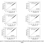
All the equations in the center of the line of this sections present the discharge coefficient through using the experimental data presented by Kumar et al. (2011) and the MLP method for each of the presented models which consider different factors influential on predicting the discharge coefficient. Figure 3 shown the correlation analysis between the discharge coefficient obtained from the MLP model and the experimental data in the training state for different models.
It could be seen with regard to the presented graphs that all six models have been trained generally well and the performance of both networks is satisfactory regarding predicting the discharge coefficient with R2 variables close to 1. However models 1 and 4 have presented relatively better results in comparison with the other models with highest R2 values which are 0.9953 and 0.9946 respectively. It could also be seen that the values predicted by these models present relatively similar results to those obtained by the experiments in almost most of the states. The process for predicting the discharge coefficient is not the same in states which the influential parameters are considered as model 4 in such a manner that the predicted values predict the results to be lesser or greater than the actual values in different points but as it could be seen, the results presented by this model are fairly accurate to the extent where the relative error presented by this model is approximately 0.67%.
 |
|
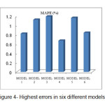
Figure 3 also shown that model 1 presents better results in comparison with the rest of the models (models 2, 3, 5, and 6). It could be seen that the process of predicting discharge coefficient in this model is almost similar to that of model 4 in such a manner that the largest relative error of prediction is nearly 0.82% in this model. Therefore it could be stated that not considering the ration of the weir crest height to the water height behind the weir ratio (L/h) does not have a significant impact on the process of predicting discharge coefficient. Model 3 presented most of the discharge- coefficient prediction results to be larger than the actual value. In such a manner that the values predicted by this model have a relative error of approximately 1.19% in some points. Therefore, it could be stated with regard to the presented explanations that not considering the Froude number (F) parameter has a significant effect on the results of predicting the discharge coefficient. Like model 3, model 5 does not predict the results with an acceptable level of accuracy either. In addition to predicting the results with greater values in comparison to the actual values, like model 3, this model predicts some values to be lesser than the actual values in some points. With regard to the relatively high degree of the relative error of these predictions, it could be stated that not considering the weir crest length to the weir length ratio (L/w) in predicting discharge coefficient decreases the prediction accuracy. Model 6 predicts discharge coefficient with an acceptable level of accuracy with a relative error of approximately 0.84%. Model 2 does not predict the results accurately either and it has a relative error of almost 1.12% in some points. Figure 4 shown the relative error presented by each of the models in predicting discharge coefficient. Carefully examining this Figure could lead to the conclusion that, model 4 has the best performance in predicting discharge coefficient of the weir flow.
 |
|
Therefore it could be stated with regard to the presented explanations that the height above the weir to the channel width ratio (h/b), the weir crest length to the weir height ration (L/W), and the approximate Froude number (F=V/√(gy)) parameters have a significant role in predicting discharge coefficient and not considering each of them decreases the prediction accuracy of the models significantly. In addition to the mentioned parameters, the vertex angle (θ) plays a role in predicting discharge coefficient as well. However as it was seen in models number 2 and 3, mot considering this parameters has no significant effect on predicting discharge coefficient and increases the value of the relative error in comparison with when this parameter is considered. With regard to the presented explanations on different models predicting discharge coefficient, Table 2 presents the prediction results of each of the models quantitatively through using different statistical indexes in training state.
Table2: Statistics Indexes - (Train)
|
Model 1 |
Model 2 |
Model 3 |
Model 4 |
Model 5 |
Model 6 |
|
|
RMSE |
0.01 |
0.013 |
0.015 |
0.009 |
0.014 |
0.011 |
|
MAPE (%) |
0.82 |
1.12 |
1.19 |
0.67 |
1.16 |
0.84 |
|
R2 |
0.99 |
0.99 |
0.98 |
0.99 |
0.98 |
0.99 |
The MAPE index is the first index which is presented for the purposes of examining the accuracy of the presented models. MAPE shows the different between the predicted values and the actual values as a percentage of the actual variables. It could be seen that the worst MAPE value was presented by model 3 which is almost 1.19%. It could also be seen that the value of this parameter is not great for any of the models. According to table two, model 4 has the least MAPE value which is almost 0.67% and it presents better results in comparison to the rest of the models with regard to this index. The RMSE index which expresses the root mean- square error has also been used to quantitatively examine the models. This index considers the weight of large errors more through exponentiation of the different between the predicted and actual values. It could be seen with regard to the table that the RMSE value is the least for model 4 in comparison to the other models. The data which were not used in the model prediction are used in this section to examine the accuracy of the presented models. The statistical indexes presented in Table 3 are used to examine the accuracy of each of the models in the testing state.
Table3: Statistics Indexes - (Test)
|
Model 1 |
Model 2 |
Model 3 |
Model 4 |
Model 5 |
Model 6 |
|
|
RMSE |
0.012 |
0.014 |
0.011 |
0.01 |
0.011 |
0.012 |
|
MAPE (%) |
1.25 |
1.62 |
1.42 |
1.14 |
1.46 |
1.4 |
|
R2 |
0.98 |
0.96 |
0.97 |
0.99 |
0.97 |
0.97 |
The value of MAPE presented by different models in the testing phase is also relatively good with the maximum value of this index which is approximately 1.62%. In this state, model 4 presents the least value of MAPE as well which is equal to 1.14% in comparison to the other models. The RMSE value which considers the root mean square of error presents the accuracy of models through considering the larger weights for larger errors. The closest this index is to zero the more accurate the model will and as it could be seen the value of this index is better in both states for model 4 in comparison with the rest of the models. Models 1 and 4 predict discharge coefficient fairly well will regard to the presented explanations however if we would like to select a model, it could be stated that model 4 presents better results.
Conclusion
There are varied methods such as using weirs for controlling flood. The weir can be located along the channel length or in the side as a side weir. The weir crest length to the water height behind the weir ratio, the weir crest length to the weir height ratio, the height of the water behind the weir to the channel width, the approximate Froude number, and the vertex angle dimensionless parameters were used in this study to predict the discharge coefficient of a weir located along the channel length. Six models were presented through considering the presented dimensionless parameters and sensitivity analysis of the different models to not using each of the varied dimensionless parameters. The examinations indicated that when all presented dimensionless parameters are used except for the weir crest length to the height of the water behind the weir (model 4) for the purposes of predicting the discharge coefficient, we will have the best results in comparison with the rest of the states. Although model 6, which does not consider the water height behind the weir to the channel width ration, also presents good results compared to model 4, the selected model (model 4) presents the discharge coefficient with an error percentage equal to 0.67% and an R2 equal to 0.9946 in the training phase of the model where its hydraulic parameters had no role in predicting the model.
Nomenclature
b Channel width (m)
Cd Coefficient of discharge
V velocity in the main channel
h the water height over the weir
g Acceleration due to gravity(m/s2)
L Crest length of water (m)
w Crest height (m)
Ï´ Vertex angle (rad)
Y head over the crest of the weir (m)
References
- Asadi, S. Shahrabi, J. Abbaszadeh, P. and Tabanmehr, S. A new hybrid artificial neural networks for rainfall-runoff process modeling. Neurocomputing, 121: 470-480(2013).
- Baghalian, S. Bonakdari, H. Nazari, F. and Fazli, M. Closed-form solution for flow field in curved channels in comparison with experimental and numerical analyses and artificial neural network. Engineering Applications of Computational Fluid Mechanics, 6(4): 514-526(2012).
- Bilgil, and Altun H. investigation of flow resistance in smooth open channels using artificial neural networks. flow measurement and instrumentation, 19:404-408(2008).
- Bilhan, O. Emiroglu, M. E. and O. Kisi. Use of artificial neural networks for prediction of discharge coefficient of triangular labyrinth side weir in curved channels. Advances in Engineering Software, 42(4): 208-214(2011).
- Bilhan, O. Emiroglu, M. E. and Kisi, O. Application of two different neural network techniques to lateral discharge over rectangular side weirs located on a straight channel. Advances in Engineering Software, 41(6):831–837(2010).
- Bonakdari, H. Baghalian, S. Nazari, F. and Fazti, M. Numerical analysis and prediction of the velocity field in curved open channel using artificial neural network and genetic Algorithm. Engineering Applications of Computational Fluid Mechanics, 5(3): 384-396(2011).
- Borghei, S. M. and Parvaneh, Discharge characteristics of a modified oblique side weir in subcritical flow. Journal of flow measurement and instrumentation, 22(5):370-376(2011).
- De Marchi, G. (1934), Saggio di teoria di fuzionamente degli stra-mazzi laterali. L’Energia Elettrica, Millano, Italy, 11(1): 849-863(2011).
- Donmez, S. Using artificial neural networks for prediction of alternate depth shaped on rectangular channel in open channel flow. Energy Education Science and Technology Part A: Energy Science and Research, 28(1): 339-348(2011).
- Dursun, O. F. Kaya, N. and Firat, M. Estimating discharge coefficient of semi-elliptical side weir using ANFIS. Journal of Hydrology, 426(3): 55-62(2012).
- Emiroglu, M. E. Kisi, O. and Bilhan, O. Predicting discharge capacity of triangular labyrinth side weir located on a straight channel by using an adaptive neuro-fuzzy technique. Advances in Engineering Software, 41(2):154–160(2009).
- Emiroglu, M. E. Kaya N. and Agaccioglu, H. Discharge capacity of labyrinth side weir located on a straight channel. Journal of Irrigation and Drainage Engineering, 136(1): 37-46(2010).
- Emiroglu, M. E. and Baylar, A. Influence of included angle and sill slope on air entrainment of triangular planform labyrinth weirs. ASCE Journal of Hydraulic Engineering, 131(3):184–9(2005).
- Huai, W. Chen, G. and Zeng, Y. Predicting apparent shear stress in prismatic compound open channels using artificial neural networks. Journal of Hydroinformatics, 15(1): 138-146(2013).
- Karimi, S. Bonakdari, H. and Gholami, A. Numerical examination of the effect of the location of flowmeters in intakes on flow velocity measurement accuracy . Bulletin of Environment, Pharmacology and life sciences, 4(7):10-27(2015).
- Kisi, O. River flow forecasting and estimation using different artificial neural network techniques. Hydrology Research, 39(1):27-40(2008).
- Kisi, O. Emiroglu, M. E. Bilhan, O. and Guven, A. Prediction of lateral discharge over triangular labyrinth side weirs under subcritical conditions using soft computing approaches. Expert Systems with Applications, 39(3):3454–3460(2012).
- Kumar, S. Ahmad, Z. and Mansoor, T. A new approach to improve the discharging capacity of sharp-crested triangular plan form weirs. Journal of Flow Measurement and Instrumentation, 22(3): 175–180(2011).
- Melesse, A. Ahmad, S. McClain, M. Wang, X. and Lim, Y. Suspended sediment load prediction of river systems: An artificial neural network approach. Agricultural Water Management, 98(5): 855-866(2011).
- Smith, M. Neural networks for statistical modeling, (Thomson Learning, 1993).
- Subramanya, K. and Awasthy, S.C. Spatially varied flow over side-weirs. Journal of the Hydraulics Division, 98(1): 1-13(1972).
- Van Maanen, B. Coco, G. Bryan, K. R. and Ruessink, B. G. The use of artificial neural networks to analyze and predict alongshore sediment transport. Nonlinear Processes in Geophysics, 17(5): 395-404(2010).
- Wormleaton, P. R. and Tsang, C. C. Aeration performance of rectangular planform labyrinth weirs. ASCE Journal of Environmental Engineering, 126(5):456–65(2000).
- Yang, H. C. and Chang, F. J. Modelling combined open channel flow by artificial neural networks. Hydrological Processes, 19(18): 3747-3762(2005).


