Climate Change Impact Assessment for Aji Basin Using Statistical Downscaling and Bias Correction of Climate Model Outputs
N. S. Vithlani1 * and H. D. Rank1
1
College of Agricultural Engineering and Technology,
Junagadh Agricultural University,
Junagadh,
India
http://dx.doi.org/10.12944/CWE.11.2.40
For the future projections Global climate models (GCMs) enable development of climate projections and relate greenhouse gas forcing to future potential climate states. When focusing it on smaller scales it exhibit some limitations to overcome this problem, regional climate models (RCMs) and other downscaling methods have been developed. To ensure statistics of the downscaled output matched the corresponding statistics of the observed data, bias correction was used. Quantify future changes of climate extremes were analyzed, based on these downscaled data from two RCMs grid points. Subset of indices and models, results of bias corrected model output and raw for the present day climate were compared with observation, which demonstrated that bias correction is important for RCM outputs. Bias correction directed agreements of extreme climate indices for future climate it does not correct for lag inverse autocorrelation and fraction of wet and dry days. But, it was observed that adjusting both the biases in the mean and variability, relatively simple non-linear correction, leads to better reproduction of observed extreme daily and multi-daily precipitation amounts. Due to climate change temperature and precipitation will increased day by day.
Copy the following to cite this article:
Vithlani N. S, Rank H. D. Climate Change Impact Assessment for Aji Basin Using Statistical Downscaling and Bias Correction of Climate Model Outputs. Curr World Environ 2016;11(2) DOI:http://dx.doi.org/10.12944/CWE.11.2.40
Copy the following to cite this URL:
Vithlani N. S, Rank H. D. Climate Change Impact Assessment for Aji Basin Using Statistical Downscaling and Bias Correction of Climate Model Outputs. Curr World Environ 2016;11(2). Available from: http://www.cwejournal.org/?p=15082
Download article (pdf) Citation Manager Publish History
Introduction
Now a days most serious challenges faced by mankind is climate change. For the assessment of future variations in the hydrologic cycle, the sensitivity of regional hydrology to variable climate conditions makes climate-change projections essential. Validation of future climate change prediction it is important to investigate observed change in present climate and can be put into context. Information gap that is provided by climate can be linked by Bias correction methods. For climate impact research, and simulation of data statistical downscaling is broadly applicable.2,4,5,10 During the historical reference period it facilitates the comparison of simulated and observed impacts and a continuous transition into the future. Bias correction helps to adjust the simulated climate data to the more detailed altitude-stratified information related with observational data. Conversely, there are several limitations of statistical bias correction like. When applying the bias correction to future periods, Stationary in bias in the historical data with respect to future data is assumed, which introduces additional uncertainty.7 The quality of the bias-corrected simulation data, is limited by both the observational dataset and the exemplification of physical processes.8
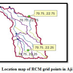
Methodology (Study area-Aji river basin)
Saurashtra has over 100 river basins; among these– Bhadar, Aji, Shatrunji and Machchhu. Aji is the most important river of Saurashtra. Average annual rainfall for Rajkot district is 552 mm for the years1961-2007. The Aji river passes through the city of Rajkot. It is situated between latitude 21ºto 22º N and longitude of 70ºto 71º E. Aji river length is 164 km with 2130 km2 catchment area. Some of the major tributaries of Aji are the Nyari, Lalapari, Khokaldadi, Banked and the Dondi. The River originating from hills of sardhar near Atkot, to its mouth at the Gulf of Kutch in Ranjitpara of Jamnagar district. There are four dams on Aji River.
 |
|
Climate Input Data
The daily temperature and rainfall data simulated by CGCM 2.3.2 for two grid points falling in/nearby Aji basin were used for the bias correction and were used based on the represented area using theissen polygon method. The weather data for the future scenarios were 2046-64 and 2081-2100. The hydrological and meteorological data like daily rainfall data, temperature (Max. and Min.) were collected from Meteorological Observatory of Main Dry land Agricultural Research Station, JAU, Targhadiya and State Water Data Center; Gandhinagar. The hydro meteorological data for the future scenarios were obtained from the IITM, Pune. The weather data was obtained through.1,3
|
Data |
Control period& Observed data |
|
Temperature (min & max) |
1/1/1978 to 31/12/2000 |
|
Precipitation |
1/1/1981 to 31/12/2000 |
The trend-preserving Bias Correction Methods
Employing transformation algorithm, correcting systematic error in RCMs grid point simulated climate variables called bias correction methods. Out of six bias correction methods are employed to adjust RCMs grid points simulations a power transformation method was used for the precipitations data and liner scaling and variance scaling were used for the temperature data.9,6,7
Bias Correction of Monthly Mean Data of Temperature (Maximum and Minimum)
Adjustment done for observed monthly mean data and long-term differences between the simulated data during the historical period and unchanged daily variability about the monthly mean.
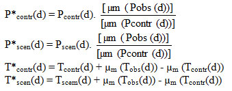
Linear Scaling of Precipitation and Temperature
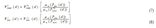
Monthly correction based on differences between observed and present-day simulated values this approach works.12
Where,
P*contr(d) = Final bias corrected daily precipitation for RCM simulated 1978-2000.
P*scen(d) = Final bias corrected daily precipitation for RCM simulated 2046-64 and 2081-2100
Pcontr(d) = Daily precipitation for RCM simulated 1978-2000.
Pscen (d) = Daily precipitation for RCM simulated 2046-2064 and 2081-2100
T*contr(d) = Final bias corrected daily Temperature for RCM simulated 1978-2000
T*scen(d) = Final bias corrected daily Temperature for RCM simulated 2046-2064 and 2081-2100. And µm = mean within monthly interval.
Pobs(d) = Daily precipitation for Observed data 1978-2000.
Tobs(d) = Daily Temperature for Observed data 1978-2000.
Power Transformation of Precipitation
A non linear correction in an exponential form a, Pb11,12,13 can be used to specifically adjust the variance statistics of a precipitation time series because it does not allow differences in the variance to be corrected. First, b is identified by matching the coefficient of variation (CV) of the corrected daily RCM precipitation (Pb) with the CV of observed daily precipitation (Pobs) for each month m: find bmsuch that
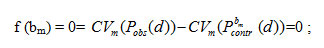
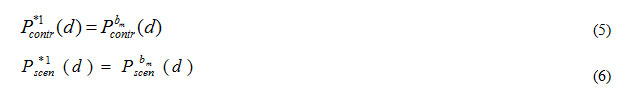
Using Brent’s method8it is done with a root-finding algorithm. Long-term monthly mean of observed precipitation matched with the monthly mean of the intermediary series P*1contr(d) by using standard linear scaling parameter:
Thus, scaling parameter depends on b, but not vice versa 12.
Variance Scaling of Temperature
Power transformation is an effective method to correct both the mean and the variance, but is limited to precipitation time series. Another approach to correct both the mean and the variance of temperature time series stepwise was presented by.11,12,13 Means of the RCM-simulated time series are adjusted by linear scaling (Eq. (3) and (4)). The mean-corrected control(T-1control (d)) and scenario runs (T-1scen (d)) are shifted on a monthly basis to a zero mean.
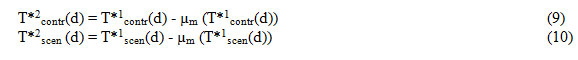
Then, the standard deviations ( σ of the shifted time seriesT*2contr(d) and T*2scen (d))are scaled based on the ratio of observed r and controlrunσ.
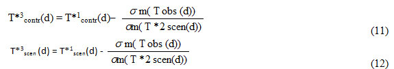
And finally, the r-corrected time T*3contr(d) and T*3scen (d) are shifted back using the corrected mean µm (T*1contr(d)) and µm (T*1scen(d)) of step one:

Results and Discussions
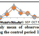
Precipitation for Control Scenario (1981-2000)
The Figure 2shows that the monthly mean of RCMs simulated precipitation higher than that of observed during monsoon months indicating over estimation by CGCM 2.3.2 RCM. The raw RCMs precipitation had a positive (Over Estimated) bias from June to August. However, for the rest of the months, the RCM simulation was matched closely with observation. In fact, after bias correction, the RCM simulated precipitation was exactly matched with observation. It indicates that the power transformation method of the bias correction of RCM simulated precipitation is good for correcting the mean precipitation.
 |
|
 |
|
Figure 3 depicts the comparison of the coefficient-a and exponent-b for correcting the biases in the mean and CV of RCM simulated daily precipitation on monthly window by comparing with actual observation during the control period. Figure 3 shows that the RCM simulated precipitation has less variability than actual observation during June to November months. The variability of the daily rainfall simulated during the rest of the months was well matched with that of observation.
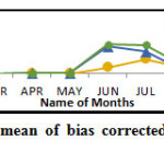
Precipitation for Future Scenarios (2046-2064 and 2081-2100)
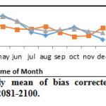
It was observed that RCMs has predicted a higher precipitation during April, May, June and July months for both scenarios.In fact, for the rest of the months, the corrected and un corrected monthly daily mean precipitation was found nearly equal. After bias correction, the precipitation amounts were reduced during monsoon months. The highest daily mean precipitation was found as 14.35mm/day in June during future scenario-2046-64 and 14.56mm/day in July during future scenario-2081-2100Fig.4(a ,b)
 |
|
Precipitation for Overall Scenarios (1961-2000), (2046-2064), (2081-2100)
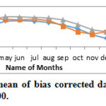
Comparison of monthly mean of bias corrected daily precipitation during 1961-2000, 2046-64 and 1981-2100 is depicted in Figure 5. It can be seen that the precipitation will increase in the future as compared to past.
 |
|
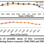
Minimum Temperature for Control Scenario (1978-2000)
 |
|
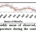
The Figure 6 shows that the monthly mean of RCMs simulated precipitation higher than that of observed during monsoon months indicating over estimation by CGCM 2.3.2 RCM. The raw RCMs simulated are still overestimated (Positive bias) during January to June months. However, for the rest of the months, the RCM simulation was matched closely with observation. In fact, after bias correction, the RCM simulated minimum temperature was exactly matched with observation.
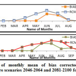
Minimum Temperature for Future Scenarios (2046-2064 and 2081-2100)
 |
|
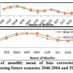
When the analysis was performed using raw data without bias correction, RCMs showed a large amount of disagreements (January-July) for both scenarios.
Minimum Temperature for Overall Scenarios (1961-2000, 2046-2064, 2081-2100)
Overall we showed that the Temperature is increased day by day due to global warming. And its directly affected to the climate change impact(Fig.8).
 |
|
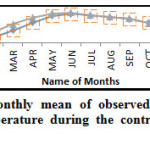
Maximum Temperature for Control Scenario (1978-2000)
Figure 9 shows that the RCMs simulated are still overestimated (positive bias) during January-April and underestimated (negative bias) during May, June, July months.
 |
|
Maximum Temperature for Future Scenarios (2046-64, 2081-2100)
 |
|
It can be seen that the RCMs simulated the higher maximum temperature during February, March and September while lower during May-July, and November-December. During the rest of the months, the uncorrected maximum temperature did agree with the bias corrected. The maximum positive bias was found during March while that of highest negative was found during June month during 2046-64.(fig.10(a)).
While in 2081-2100 it can be seen that the RCMs simulated the maximum temperature higher during January-April and August-September while lower during rest of the months. (Fig. 10(a, b)).
Maximum Temperature for Overall Scenario (1961-2000, 2046-2064, 2081-2100)
 |
|
Fig.11 Shows that the highest increase in the maximum temperature in the future can be during the December to March. This can affects the cereal crops sown during the winter season.
Conclusions
Temperature and precipitation RCM is strongly dependent on the choice of the correction algorithm, both for current and future climate conditions. For the monthly mean values the linear-scaling approach offers corrected data with variability more consistent with the original RCM data. It is furthermore not able to correct frequencies. For the variance and the mean of raw RCM data the power transformation and variance scaling adjusts both. They perform much better than the previous approaches in terms of correcting several statistical characteristics and in terms of the variability range. Although the power transformation corrects the coefficient of variation and percentiles to some extent, it does not provide corrected RCM data with accurate probability of dry day sand precipitation intensity. As a result, this nonlinear transformation may do less well for RCM simulations having a larger bias in the wet-day frequency.11,13 The potential changes of the surface climate over the Aji river basin based on a two RCMs grid points driven by GCMs have been examined in this study. Results of simulations using the regional climate model, for the control period and likely future climate were analyzed to develop an understanding as to how climate extremes may change in the Aji river basin. Results showed that the annual average rainfall was found increased from 358 mm during 1961-2000 to 575mm during 2046-64 to 928mm during 2081-2100. Annual average maximum temperature was found increased from 33.89 oC during 1961-2000 to 35.33 oC during 2046-64 to 35.87 oC during 2081-2100. Annual average minimum temperature was found increased from 19.51 oC during 1961-2000 to 22.15 oC during 2046-64 to 25.43 oC during 2081-2100.
References
- Dile, Y.T., Srinivasan R. Evaluation of CFSR climate data for hydrologic prediction in data scare watersheds: an application in the Blue Nile river basin. Journal of the American water resources association(JAWRA):1-16 (2014).
- Ehret, U., Zehe, E., Wulfmeyer, V., Warrach-Sagi, K., and Liebert, J. HESS Opinions “Should we apply bias correction to global and regional climate model data? Earth Syst. Sci., 16: 3391–3404 (2012).
CrossRef - Fuka, D.R., C.A. Mcallister, A.T. Degaetano and Eastern Z.M. Using the climate forecast system reanalysis dataset to improve weather input data for watershed models. Proc. (2013).
- Hagemann, S., Chen, C., Haerter, J. O., Heinke, J., Gerten, D., and Piani, C. Impact of a statistical bias correction on the projected hydrological changes obtained from three GCMs and two hydrology models. Hydrometeorol., 12: 556–578 (2011).
CrossRef - Ines, A. V. and Hansen, J. W. Bias correction of daily GCM rainfall for crop simulation studies. Forest Meteorol. 138: 44–53(2006).
CrossRef - Maraun, D. Bias Correction, Quantile Mapping, and Downscaling: Revisiting the Inflation Issue. Climate, 26: 2137–2143 (2013).
CrossRef - Maraun, D. Non stationarities of regional climate model biases in European seasonal mean temperature and precipitation sums. Res. Lett. 39: 1–5 (2012).
CrossRef - Maraun, D., Wetterhall, F., Ireson, A. M., Chandler, R. E., Kendon,E. J.,Widmann, M., Brienen, S., Rust, H.W., Sauter, T., Theme ßl, M., Venema, V. K. C., Chun, K. P., Goodess, C. M., Jones, R. G.,Onof, C., Vrac, M., and Thile-Eich, I. Precipitation down scalingunder climate change. Recent developments to bridge the gap between dynamical models and the end user. Geophys., 48. (2010).
- Piani, C. and Haerter, J. O. Two dimensional bias correction of temperature and precipitation copulas in climate models. Res. Let. 39. (2012).
- Robock, A., Turco, R., Harwell, M., Ackerman, T., Andressen, R., Chang, H.-S. and Sivakumar, M. Use of general circulation model output in the creation of climate change scenarios for impact analysis. Change, 23: 293–335 (1993).
CrossRef - Leander, R., Buishand, T.A. Resampling of regional climate model output forthe simulation of extreme river flows. Hydrol. 332 (3–4):487–496(2007).
CrossRef - Leander, R., Buishand, T.A., van den Hurk, B.J.J.M., de Wit, M.J.M. Estimated changes in flood quintiles of the river Meuse from resampling of regional climate model output. Hydrol. 351 (3–4):331–343(2008).
CrossRef - Teutschbein, Claudia, and Jan Seibert. "Bias correction of regional climate model simulations for hydrological climate change impact studies: Review and evaluation of different methods", Journal of Hydrology, 2012.
CrossRef


