Evaluation of Evapotranspiration Estimation Models for Junagadh City of Gujarat
H.H. Mashru1 and D.K. Dwivedi1 *
1
Department of Soil and Water Engineering,
College of Agricultural Engineering and Technology,
Junagadh Agricultural University (JAU),
Junagadh,
India
http://dx.doi.org/10.12944/CWE.11.2.34
Estimation of Evapotranspiration is important for determining the agro-climatic potential of a particular region, water requirement of field crops, irrigation scheduling and suitability of crops or varieties, which can be grown successfully with the best economic returns and therefore numerous models have been developed for determining evapotranspiration. The performance evaluation of commonly used reference evapotranspiration (ET0) estimation methods like FAO 56 Penman-Monteith, Samani and Hargreaves, Makkink, Blaney Criddle, Jensen-Haise, Priestly-Taylor, FAO 24 radiation and Modified Penman Monteith method based on their accuracy of estimation has been undertaken in this study. The inter-relationship between FAO-56 Penman-Monteith method and other reference evapotranspiration (ET0) estimation method is also determined in this study. The results showed that Blaney Criddle method, Modified Penman method, Jensen-Haise method and Priestly-Taylor method are the alternative methods to Penman-Monteith method for better estimate of ET0 for the Junagadh city of Gujarat, India.
Copy the following to cite this article:
Mashru H. H, Dwivedi D. K. Evaluation of Evapotranspiration Estimation Models for Junagadh City of Gujarat. Curr World Environ 2016;11(2) DOI:http://dx.doi.org/10.12944/CWE.11.2.34
Copy the following to cite this URL:
Mashru H. H, Dwivedi D. K. Evaluation of Evapotranspiration Estimation Models for Junagadh City of Gujarat. Curr World Environ 2016;11(2). Available from: http://www.cwejournal.org/?p=15061
Download article (pdf) Citation Manager Publish History
Introduction
Evapotranspiration is one of the important phases of hydrologic cycle and its accurate estimation is of paramount importance for water balance studies, irrigation system design, crop yield simulation and water resources planning and management. The Penman-Monteith method recommended by UN - FAO has received widespread acceptance internationally for estimating ET0. However, the major limitation of the method is that it requires data for a large number of weather parameters, which may not be available for many locations.
Evapotranspiration process is the combination of two separate processes commonly known as Evaporation and Transpiration. In this process water is lost on the one hand from the top soil or water surface by evaporation and on the other hand from the crop plant tissues through transpiration by stomatal dynamics.
Evaporation and transpiration occur simultaneously therefore there is no easy way of distinguishing between the two processes. Instead of water quantity in the topsoil, the evaporation from a cropped soil is mainly determined by the fraction of the solar radiation reaching the soil surface. When the crop is small, water is predominately lost by evaporation from the soil surface, but once the crop is well developed and completely covers the soil, transpiration becomes the main process
Estimates of evapotranspiration provide an outlook of soil water balance in association with the amount of precipitation. Such estimates are of immense importance for calculation of water demand of the field crops and irrigation scheduling. It also determines the nature of agro-climate a region has, agro-climatic potential of that region and suitability of crops or varieties, which can be grown successfully with the best economic returns.
Many scientists developed mathematical equations to estimate evapotranspiration in different parts of the world but no one can be universally recommended and adopted. To allow for greater understanding, sharing, and comparison of evapotranspiration information worldwide, under varying climatic and agronomic conditions, a standardized method of estimating ETo was developed referred to as the FAO-56 Penman-Monteith method.
The concept of a reference evapotranspiration (ETo) can be used to estimate the climatic effect on evapotranspiration and represents the evapotranspiration from a hypothetical, reference surface. Many equations are used to estimate ETo which be divided into two main groups, i) those that are empirical and have lower data requirements, and ii) those that are physically-based and require proportionately more data. The present study focused to the performance evaluation of commonly used ET0 estimation methods based on their accuracy of estimation and development of inter-relationships between the Penman-Monteith and the other climatological methods.
Objectives
- To evaluate the various evapotranspiration estimation method
- To develop inter-relationship between FAO-56 Penman-Monteith method and other ET0 estimation method.
Materials and Methods
The daily records of meteorological parameters i.e. Maximum temperature (Tmax), minimum temperature (Tmin), relative humidity morning (RH1), relative humidity evening (RH2), wind speed (WV), bright sunshine hours (BSS) and Pan evaporation (EP) recorded for the period of 10 years (year 2005 to year 2015) were collected from Meteorological department, Junagadh Agricultural University, Junagadh. The daily data was further converted into the monthly data. Standard methods as mentioned below were used to estimate ETo.
Evapotranspiration Estimation Methods
There are eight ET estimation methods were used to estimate the evapotranspiration i.e. FAO 56 Penman-Monteith, Samani and Hargreaves, Makkink method, Blaney Criddle method, Jensen-haise method, Priestly-Taylor method, FAO 24 radiation method and Modified Penman Monteith method. Description of each method is provided in the following sections.
FAO 56 Penman-Monteith Method (PMM)
The FAO Penman-Monteith method is a physically-based analytical approach derived from the Penman-Monteith equation,5 a combination of the energy balance and mass transfer method, specifying the resistance factors of the reference surface. It defines the reference surface as a hypothetical surface of green grass with an assumed uniform height of 0.12 m, a surface resistance of 70 s m-1 and an albedo of 0.23 under actively growing and adequately watered conditions.1 The FAO Penman-Monteith method to estimate ETo is derived as:
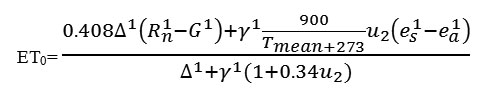
Where,
ETo = reference evapotranspiration [mm day-1],
Rn = net radiation at the surface [MJ m-2 day-1],
G = soil heat flux density [MJ m-2 day-1],
T = air temperature at 2 m height [°C],
u2 = wind speed at 2 m height [m s-1],
es = saturation vapour pressure [kPa],
ea = actual vapour pressure [kPa],
Δ = slope of vapour pressure curve [kPa °C-1],
Γ = psychrometric constant [kPa °C-1].
Ë =0.000665*p(kpa)
Ea=(e(min)*(rhmax/100)+e(max)*(rhmin/100))/2
U2=ws*4.87*1000/(3600*emin(67.8*3-5.42))
J=1,2,3…….
G=0
Site location information of altitude and latitude and standard climatological records of solar radiation, air temperature, relative humidity and wind speed are required. Altitude and latitude of the site location are needed to adjust the local psychometric constant (γ) and latitude is also involved in extra-terrestrial radiation (Ra) computation. Solar radiation is required to calculate Rn based on a radiation balance model in combination with Ra. T is used to develop Δ and calculate vapour pressure deficit (VPD). To ensure the integrity of ETo estimation, all the climatological parameters should be measured at 2 m or converted to this height.1
FAO 56 Hargreaves Method (HRM)
The Samani and Hargreaves method is a temperature-based empirical approach.11 It was developed from the Christiansen equation,7 which uses a multiplicative method to relate ET to solar radiation, temperature, relative humidity and wind speed, respectively. In an experiment conducted by Hargreaves9 on a cool season grass region at Davis, Calif., regressions were made using ET measurements as a function of various combinations of weather factors and showed that the multiplication of temperature by solar radiation explains 94% of variability of ET measurements and that of wind speed by relative humidity only explains about 10%. Based on these results, coefficients for wind speed and relative humidity were left out of the equation to foster simplicity and reduce data requirements. Currently the Hargreaves and Samani method is generally described as:
ET0 =0.0023Ra(T mean+ 17.8)*(T D )0.5
Where,
ETo = reference evapotranspiration [mm day-1],
Tmean = mean daily air temperature at 2 m height [°C],
Tmax = daily maximum temperature at 2 m height [°C],
Tmin = daily minimum temperature at 2 m height [°C],
Ra = extraterrestrial radiation [MJ m-2 day-1].
TD =Tmax-Tmin
Ra=(24*60/3.14)*0.82*dr*(ws*sin(lati.(rad)*sin(del)+cos(lati.(rad)*cos(lati.(rad)*sin(ws))
Due to the low data requirement, it is often applied under conditions where less data is available, and especially, when only air temperatures are available.10 It is also used to estimate historical series of ET in irrigation and water resources systems, using historical air temperature records,20
FAO 24 Radiation Method (RAM)
The FAO 24 Radiation method was first introduced by Doorenbos and Pruitt (1977) as a modification of the Makkink (1957) method5,13 It was originally suggested that this model be used over a Penman method when measured air temperature and solar radiation were available but wind and humidity data were unavailable or were of questionable quality.5,15 However, the 24RD model performs much better with measured data.13 The form of 24RD given by Jensen et al. (1990) is described in equation:
ET0 =c(W*Rs)
Where,
c=1.066-0.00128RHmean+0.045ud-0.0002RHmeanud+0.0000315(RHmean)2-0.00103(ud)2
Δ=(4098*(o.6108*exp((17.27*tmean)/(tmean+237.3))))/((tmean+237.3)
Ë =0.000665*p(kpa)
G=0
Rn=Rns-Rnl
where ETo is grass-reference evapotranspiration (mm day-1), and are the same variables defined for Equation 3.1, Rs is solar radiation (mm day-1) (see [2] for conversion factors), and a = -0.3 mm day-1 where RHmean is the daily mean relative humidity (percent) and Ud is the mean daytime wind speed (m s-1).13
FAO 24 Blaney-Criddle Method (BCM)
Blaney and Criddle (1950) developed their model for use in arid farmlands of the western U.S. while working as engineers for the Soil Conservation Service (SCS).12 The model’s relationships were derived from experimental data for a variety of crops over the western U.S.6 The original model is similar to the classic Thornthwaite model, requiring only temperature and a function of sunlight hours as data input. The original model as described by Blaney and Criddle (1950) is:
ET0 =a+b
Where,
a =0.0043(RHmin)-n/N-1.41
b =0.82-0.0041(RHmin)+1.07(n/N)+0.066(ud)-0.006(RHmin)(n/N)-0.0006(RHmin)(ud)
lati(rad)=lati.*3.14/180
del=0.409*sin((2*3.14*j/365)-1.39)
ws=acos(-tan(lati.(rad)*tan(del))
with T being the mean monthly temperature (°F) and P the monthly percentage of the annual daytime hours.6
where ETo is reference evapotranspiration (mm day-1), p is the mean percentage of annual daytime hours (defined as the percentage of the total annual daylight hours that occur in the time period being examined, such as daily or monthly,8 T is the mean air temperature (°C), RHmin is the minimum relative humidity (percent), n/N is the ratio of possible to actual sunshine hours, and Ud is the daytime wind speed at 2 m (m s-1). The original Blaney- Criddle model was designed to use monthly values only and was known to produce erroneous results for any period shorter than one month.12 This limitation was due to the use of temperature as the sole climatic variable.12 The 24BC version of the model, however, uses humidity and wind speed, thus minimizing this limitation.
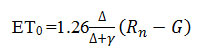
Priestley-Taylor Method (PTM)
The original intent of the model was for use in large-scale numerical modeling where it is assumed that advection is small, thus allowing the aerodynamic component of the original Penman equation to be reduced to a coefficient that modifies the remaining equation (Priestley and Taylor 1972, Jensen et al. 1990). The P/T model was designed to be used in humid areas where surfaces were usually wet.19,13 The form of the P/T used in this study was described by Jensen et al. (1990) as:
Δ=(4098*(o.6108*exp((17.27*tmean)/(tmean+237.3))))/((tmean+237.3)
Ë =0.000665*p(kpa)
G=0
Rn=Rns-Rnl
where ET is evapotranspiration (mm day-1) and all other terms are identical to those defined previously. The coefficient term may be modified for different wind and humidity regimes, but it has been found that the current value of 1.26 is reasonable across most climates.17
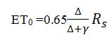
Makkink Method (MKM)
The Makkink model was designed in 1957 in the Netherlands as a modification of Penman after comparing the Penman model to lysimetric data.10,16 Currently, Makkink is popular in western Europe10 and has been used successfully in the U.S.4 Allen gave the operational form of the Makkink model as:
Δ=(4098*(o.6108*exp((17.27*tmean)/(tmean+237.3))))/((tmean+237.3)
Rs=(o.25+0.5*(n(hrs)/n))*ra^2
Ë =0.000665*p(kpa)
Where ETo is evapotranspiration (mm day-1), Rs is solar radiation (MJ m-2 day-1), and are the same variables defined for Equation.
Modified Penman Method (MPM)
The equation formed as a result of combination of radiation term and aerodynamic term which is given as:
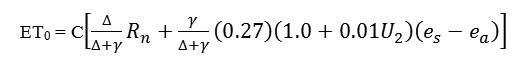
Where,
C=0.68+0.0028(RHmax)+0.018(Rs)- 0.068(ud)+0.013(ud/un)+0.0097(ud)(ud/un)+0.000043(RHmax)(Rs)(ud)
Where,
ETo = Reference crop evapotranspiration in mm/day
W = Temperature related weighing factor.
Rn = Net radiation equivalent evaporation in mm/day.
f(u) = Wind related function
Δ= (4098*(o.6108*exp((17.27*tmean)/(tmean+237.3))))/((tmean+237.3)
Rs = (o.25+0.5*(n(hrs)/n))*ra^2
Es = (Tmax+Tmin)/2
(es-ed) = Difference between saturated vapor pressure at mean air temperature and the actual vapor pressure of the air, in mille-bar.
C = Adjustment factor to compensate for the effect of day and night
Jensen-Haise Method (JHM)
The Jensen-Haise model is essentially a shortened version of the original Penman combination equation. The original intent of the model was for use in large-scale numerical modelling. The equation is given as:
ET01 =Rs(0.025Tmean+0.08)
Where,
T mean=mean daily temperature,
Rs =global solar radiation, mm/day
Rs=(o.25+0.5*(n(hrs)/n))*ra^2
Table 1: Percent Deviations of Average Monthly Et0 Values Estimated by Various Methods with Penman Monteith Method
|
Method Month |
BCM |
JHM |
HRM |
PTM |
RAM |
MKM |
MPM |
|
1-J |
20.34 |
220.49 |
220.21 |
353.21 |
254.89 |
113.53 |
228.18 |
|
2 |
25.44 |
238.21 |
231.77 |
367.58 |
268.93 |
122.02 |
241.82 |
|
3 |
26.04 |
252.81 |
267.95 |
389.49 |
284.82 |
131.50 |
257.73 |
|
4 |
35.00 |
229.44 |
225.13 |
366.45 |
266.46 |
122.42 |
234.82 |
|
5 |
26.53 |
239.57 |
217.95 |
383.41 |
284.39 |
132.30 |
254.07 |
|
6-F |
44.38 |
220.76 |
191.17 |
354.06 |
261.66 |
118.50 |
230.01 |
|
7 |
40.88 |
226.41 |
198.72 |
345.43 |
255.25 |
114.87 |
222.82 |
|
8 |
53.52 |
224.55 |
203.t88 |
337.64 |
248.45 |
112.12 |
215.75 |
|
9 |
56.28 |
219.51 |
183.48 |
327.21 |
242.15 |
108.34 |
210.04 |
|
10-M |
63.81 |
213.98 |
170.35 |
322.50 |
239.13 |
106.12 |
207.77 |
|
11 |
46.96 |
209.61 |
150.34 |
307.01 |
228.00 |
100.44 |
191.79 |
|
12 |
56.26 |
222.56 |
166.36 |
296.46 |
220.69 |
94.59 |
191.10 |
|
13 |
46.35 |
233.30 |
174.48 |
296.63 |
221.01 |
95.23 |
187.45 |
|
14-A |
65.66 |
209.16 |
173.11 |
263.28 |
193.60 |
78.47 |
162.04 |
|
15 |
56.79 |
221.11 |
181.37 |
277.48 |
206.43 |
85.38 |
177.21 |
|
16 |
51.09 |
212.58 |
156.51 |
263.56 |
197.16 |
79.09 |
165.93 |
|
17 |
56.90 |
218.94 |
159.88 |
266.88 |
201.91 |
81.65 |
173.14 |
|
18 |
57.88 |
203.59 |
121.56 |
259.34 |
197.19 |
77.28 |
168.24 |
|
19-M |
50.81 |
207.68 |
133.44 |
256.39 |
196.22 |
75.47 |
165.84 |
|
20 |
45.29 |
225.40 |
133.59 |
260.18 |
201.94 |
77.80 |
168.82 |
|
21 |
39.27 |
184.18 |
121.58 |
221.67 |
168.10 |
57.70 |
137.79 |
|
22 |
38.74 |
194.35 |
133.14 |
227.03 |
172.14 |
60.45 |
139.51 |
|
23-J |
12.05 |
174.75 |
140.59 |
209.26 |
156.18 |
50.15 |
124.33 |
|
24 |
-19.72 |
207.53 |
193.42 |
253.64 |
198.39 |
71.17 |
158.01 |
|
25 |
8.79 |
164.06 |
180.19 |
200.04 |
148.31 |
42.89 |
115.09 |
|
26 |
-12.45 |
165.57 |
219.85 |
206.26 |
152.67 |
42.41 |
115.50 |
|
27-J |
-0.79 |
216.92 |
290.81 |
261.46 |
201.68 |
67.39 |
153.35 |
|
28 |
4.96 |
203.85 |
307.11 |
245.89 |
188.39 |
59.60 |
142.24 |
|
29 |
5.01 |
220.14 |
324.00 |
261.86 |
202.80 |
68.70 |
154.44 |
|
30 |
-0.36 |
241.67 |
308.75 |
286.64 |
230.82 |
81.86 |
174.03 |
|
31 |
13.44 |
255.14 |
409.20 |
321.27 |
262.05 |
95.96 |
196.63 |
|
32-A |
15.41 |
220.36 |
379.96 |
281.92 |
225.43 |
76.93 |
166.29 |
|
33 |
11.63 |
253.83 |
369.85 |
310.36 |
254.29 |
94.49 |
190.35 |
|
34 |
18.68 |
258.97 |
348.37 |
314.12 |
260.57 |
100.92 |
198.13 |
|
35 |
35.45 |
287.01 |
374.51 |
327.44 |
277.41 |
107.95 |
206.70 |
|
36-S |
46.05 |
295.42 |
297.77 |
334.88 |
287.60 |
117.47 |
218.01 |
|
37 |
40.33 |
304.80 |
271.05 |
339.73 |
295.37 |
123.84 |
224.45 |
|
38 |
24.92 |
312.18 |
249.80 |
351.01 |
311.40 |
132.92 |
234.95 |
|
39 |
-14.04 |
327.66 |
243.78 |
362.74 |
324.67 |
141.38 |
243.68 |
|
40-O |
10.36 |
323.20 |
232.54 |
351.41 |
311.78 |
139.04 |
232.93 |
|
41 |
3.46 |
316.34 |
227.77 |
345.72 |
306.88 |
137.50 |
227.93 |
|
42 |
36.57 |
310.96 |
257.14 |
357.19 |
315.31 |
145.11 |
234.59 |
|
43 |
56.77 |
311.13 |
265.11 |
371.55 |
323.95 |
155.69 |
237.09 |
|
44 |
53.56 |
284.40 |
257.63 |
344.49 |
297.63 |
140.24 |
213.61 |
|
45-N |
41.23 |
293.36 |
257.00 |
352.28 |
307.25 |
145.07 |
219.53 |
|
46 |
35.00 |
292.20 |
273.20 |
345.26 |
302.73 |
141.75 |
214.19 |
|
47 |
39.76 |
306.57 |
296.89 |
370.02 |
328.90 |
157.95 |
234.44 |
|
48 |
22.74 |
261.39 |
246.57 |
325.38 |
287.57 |
133.83 |
198.83 |
|
49-D |
18.02 |
257.47 |
256.14 |
322.24 |
287.54 |
132.31 |
199.69 |
|
50 |
14.85 |
241.16 |
239.78 |
317.63 |
284.50 |
131.87 |
194.81 |
|
51 |
12.02 |
250.95 |
274.06 |
316.28 |
284.87 |
130.95 |
194.34 |
|
52 |
-1.07 |
226.82 |
261.17 |
306.77 |
277.13 |
126.39 |
184.50 |
Results and Discussion
Evapotranspiration Estimation Methods
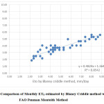
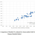
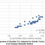
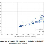
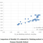
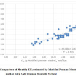
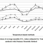
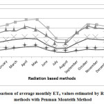
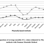
The mean monthly ETo values estimated by various methods are compared with those estimated by FAO 56 PMM as shown in Fig.1 to Fig.7. Good agreement was observed between Blaney-Criddle method, MPM, JHM, PTM and with FAO 56 Penman-Monteith Method. Results indicated that poor relationship was observed with HRM with FAO 56 Penman-Monteith Method.
The percent deviations of mean monthly ET0 values with respect to PMM are presented in Table 1. The positive deviation represents overestimation and negative deviation represents underestimation of ET0. All the ET0 estimation methods overestimated average monthly ET0 during monsoon period in the study area except Blaney criddle method. The percent deviation has increased as the monsoon progresses.
The comparison of monthly ET0 values estimated by various methods with those of PMM is presented in Fig 1. to Fig 7. Linear regression analysis has been carried out to derive inter relationships between PMM and other methods are presented in Table 2. These relationships, therefore, may be adopted to estimate ET0 by the methods for which meteorological data are available to get reasonable estimation in terms of the desired method.
Fig.1 shows the comparison of monthly ET0 estimated by Blaney Criddle method with FAO Penman Monteith method. The value of coefficient of determination was found to be 0.8542 which is higher than that obtained by other methods used in this study as shown in fig.2, fig.3, fig.4, fig.5, fig. 6 and fig.7 suggesting a strong correlation between Blaney Criddle and Penman Monteith method. The comparison of monthly ET0 estimated by Hargreaves method with FAO Penman Monteith Method as shown in fig.3 indicates that it has least value of coefficient of determination compared to other methods. As indicated in fig.1, fig.2, fig. 4 and fig.7, the value of coefficient of determination is greater than 0.7 suggesting that there is a stronger correlation of Blaney Criddle Method, Jensen-Haise Method, Priestly-Taylor Method, Modified Penman Monteith Method compared to Hargreaves Radiation Method, FAO 24 Radiation Method and Makkink Method.
 |
|
 |
|
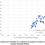 |
Figure 3: Comparison of Monthly ET0 estimated by Hargreaves method with FAO Penman Monteith Method Click here to View figure |
 |
|
 |
|
 |
|
 |
|
Table 2: Interrelationships Between Various Empirical Methods and Pmm
|
Sr. No. |
Conversion equation |
R2 |
|
1 |
PMM=0.482BCM+1.364 |
0.854 |
|
2 |
PMM=0.285JHM+0.130 |
0.763 |
|
3 |
PMM=0.493HRM-2.137 |
0.435 |
|
4 |
PMM=0.246PTM+0.025 |
0.752 |
|
5 |
PMM=0.27RAM+0.280 |
0.649 |
|
6 |
PMM=0.419MKM+0.567 |
0.649 |
|
7 |
PMM=0.328MPM+0.155 |
0.765 |
 |
|
 |
|
 |
|
Table 3: Regression Equations with Interrelationships Between Various Empirical Methods
|
Sr. No. |
Methods |
Equation |
R2 |
|
1 |
Blaney Criddle Method |
Y=0.482X+1.364 |
0.854 |
|
2 |
Jensen-Haise Method |
Y=0.285X+0.130 |
0.763 |
|
3 |
Hargreaves Radiation Method |
Y=0.493X+2.137 |
0.435 |
|
4 |
Priestly-Taylor Method |
Y=0.246X+0.025 |
0.752 |
|
5 |
FAO 24 Radiation Method |
Y=0.27X+0.280 |
0.649 |
|
6 |
Makkink Method |
Y=0.419X+0.567 |
0.649 |
|
7 |
Modified Penman Monteith Method |
Y=0.328X+0.155 |
0.765 |
|
Where Y= Penman Monteith response variable and X= Predictor variable of methods in col(2) |
|||
Conclusion
Many methods have been proposed for estimating ETo based on weather data, and range from locally developed, empirical relationships to physically based energy- and mass-transfer models. To allow for greater understanding, sharing, and inter comparison of evapotranspiration information worldwide, under varying climatic and agronomic conditions, a standardized method of estimating ETo was developed, referred to as the FAO-56 Penman-Monteith method. It is a complex method requiring several weather parameters, including air temperature, humidity, solar radiation, and wind speed, to be measured under strict conditions. Other methods were later on given by various scientists to estimate the evapotranspiration and considering this, the study was under taken to
To evaluate the various evapotranspiration estimation method
To develop inter-relationship between Penman-monteith and other ET0 estimation method.
The data was collected from the Metrological department, Junagadh Agricultural University, Junagadh
There are eight ET estimation methods were used to estimate the evapotranspiration i.e. FAO 56 Penman-Monteith, Samani and Hargreaves, Makkink, Blaney criddle, Jensen-haise, Priestly-Taylor, FAO 24 radiation and Modified Penman Monteith method. After evaluation following conclusions were drawn out of it
The BCM, MPM, JHM and PTM are the alternative methods to PMM for better estimate of ET0 for the Junagadh region of Gujarat, India.
The following inter-relationships were developed between Penman-Monteith and other ET0 estimation method.
References
- Allen, R.G., Pereira, L.S., Raes, D. & Smith, M. Crop evapotranspiration. Guidelines for computing crop water requirements. FAO Irrigation and Drainage Paper 56, Rome, Italy, 300 pp (1998).
CrossRef - Allen, R.G. Using the FAO-56 dual crop coefficient method over an irrigated region as part of an evapotranspiration inter-comparison study. Journal of Hydrology. 229, 27–41 (2000).
CrossRef - Allen, R.G., Tasumi, M. & Trezza, R. Satellite-based energy balance for mapping evapotranspiration with internalized calibration (METRIC)-model. Irrig. Drain. E., 133, 380-394 (2007).
- Amatya, D.M., Skaggs, R.W. & Gregory, J.D. Comparison of methods for estimating REF-ET. Journal of Irrigation and Drainage Engineering; 121(6): 427-435 (1995).
CrossRef - Batchelor, C.H. The accuracy of evapotranspiration functions estimated with the FAO modified Penman equation. J. Irrigation Sci. 4–5, 223–234 (1984).
- Blaney, H. F. & Criddle, W. D. Determining Water Requirements in Irrigated Area from Climatological Irrigation Data, US Department of Agriculture, Soil Conservation Service, Tech. Pap. No. 96, 48 pp (1950).
- Christiansen, J. E. Pan evaporation and evapotranspiration from climatic data.‘‘ Irrig. Drain. Div., 94, 243–265 (1968).
- Doorenbos, J. and W.O. Pruitt. Guidelines for predicting crop water requirements. FAO. Irrigation and Drainage Paper 24. Food and Agriculture Organization. Rome (1977).
- Hargreaves, G. H. Moisture availability and crop production. ASAE, 18~5, 980–984 (1975).
CrossRef - Hargreaves, G. H. & Allen, R. G.: History and evaluation of Hargreaves evapotranspiration equation, J. Irrig. Drain. Eng., 129, 53–63 (2003).
- Hargreaves, G. H. & Samani, Z. A. Estimating potential evapotranspiration, J. Irrig. Drain. Eng., 108, 225–230 (1982).
- Hansen, V.E., O.W. Israelsen, & G.E. Stringham. Irrigation Principles and Practices 4th New York, NY: John Wiley and Sons, Inc (1980).
- Jensen M.E., R.D. Burman & R.G. Allen, Evaporation and irrigation water requirements, ASCE Manuals and Reports on Eng. Practices No. 70, Am. Soc. Civil Eng., New York, NY, 360 pp (1990).
CrossRef - Jensen, C., Stougaard, B. & Olsen, P. Simulation of nitrogen dynamics at three Danish locations by use of the DAISY model. Acta Agric. Scand., Sect. B, Soil and Plant Science, 44, 75-83 (1994).
- Jensen, D. T., Hargreaves, G. H., Temesgen, B. & Allen, R. G. Computation of ETo under non ideal conditions, J. Irrig. Drain. Eng., 123, 394–400 (1997).
- Makkink, G.F. Testing the Penman formula by means of lysimeters. Journal of the Institution of Water Engineers and Scientists. Vol. 11. 277–288 (1957).
CrossRef - Mcaneney, K.J. & Itier, B. Operational limits to the Priestley-Taylor formula. Irrigation Science 17:37-43 (1996).
- Penman, H.L. Natural evaporation from open water, bare soil and grass, R. Soc. Lond., 193, 120-145 (1948).
CrossRef - Priestley, C.H.B. & Taylor, R.J. On the assessment of surface heat flux and evaporation using large scale parameters. Monthly Weather Reviews. 100: 81–92 (1972).
CrossRef - Vanderlinden, K., Gira´ldez, J.V. & Van Mervenne, M. Assessing reference evapotranspiration by the Hargreaves method in Southern Spain. J. Irrig. Drain. Eng. ASCE 129 (1), 53–63 (2004).
CrossRef


