Current World Environment

Introduction

Groundwater is the sole dependable source of consumption for drinking water, agriculture, and industry in dry and semi-dry regions. Evidently, quantity and quality of water resources during the next year is important in water resource management. Since 1950, Groundwater simulation has been used vastly for a better management of groundwater resources. Therefore, many researchers have tried to find more accurate models, considering the actual conditions. These models require plenty of information which is difficult and sometimes impossible to gather. And also, considering some execution conditions, reaching a conclusion takes more time if possible at all. On the other hand, there are numerous factors in hydrologic parameters which complicate applying data to the models. Making physical and conceptual models have been poorly noticed for difficulty of gathering more information and the required time for calibration. In addition, nonlinearity of variables makes the problem more challenging. Recently, Artificial Intelligence (AI) models, as new powerful tools, have been used for forecasting hydrologic parameters. These methods act as a black box and do not require lots of physical data and are capable of estimating non-static water quality. Due to short processing time and low input data, AI models can supersede numerical ground water models. These new methods act as powerful estimators without the need for governing equations. For error reduction in regional forecasting, all selected wells must choose from one homogeny cluster. So, it is necessary to define cluster homogeny by some examinations. But one must make sure that these places are available. Because choosing some clusters with some wells inside is not sufficient for homogeny. The L-moments as the new types of statistical methods act for solving such problems. A quick search shows that regional forecasting with ANFIS-GA is a new method for modeling. Nero-fuzzy networks for flood regional analysis were used .¹ Investigation shows that nero-fuzzy model versus artificial neural networks and non-linear correlation, has better ability in modeling of flood estimation in watersheds without hydrometer At-Sites. L-moments was investigated the great supply of four aquifers in Australia.² They found that regional analysis increase the accuracy of forecasting. Adaptive neuro fuzzy inference system (ANFIS) have been used to predict water supply in terms of quality and quantity trends in sophisticated systems with acceptable accuracy.^3,4,5,6and7 Methods of AI are nonlinear tools of modeling which do not need any explicit of the physical relationship of the problem. Through recent years, those successful applications for Soft Computing Techniques in the field of water engineering have been published in a great scale.^8,9ad10 This paper attempts forecasting regional salinity of groundwater of kerman plain by ANFIS-GA with L-moments and comparison of between regional and At-Site results.

Study Area

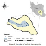
This research has been geographically focused in the aquifer of Kerman plain which is a region in Kerman province located in the south-eastern of Iran as illustrated in Figure.3. Reportedly, there is no existence of any permanent river in this plain; therefore, the water supply demands for agricultural, industrial, domestic and municipal consumption in 3200 km2 area around this plain highly depends on groundwater. Droughts and increasing pumping wells in two recent decades have mainly caused major groundwater decline which is happening at a rate of (1-3) meter per year in different wells across the area. Besides, other problems have helped the deterioration of ground water quality.¹¹ The long-term annual precipitation for this area has noticeably decreased from 150 to 100 (mm/year) in the last 20 years (1993-2013).The local acquired data consists (time series/frequency) of rainfall and ground water levels measured at Kerman airport At-Site (latitude: 30o, 16' N, longitude: 56o, 54’ E). The data set was collected by the Iranian Ministry of Energy.⁸

Materials and Methods

L-moments

(Hosking, 1990) has a new definition of L-moments. Based on his studies, L-moments are analogous to traditional moments which are expressible as linear combinations of order statistics. Basically L-moments have linear functions as probability-weighted moments (PWMs).¹² Alike conventional moments, the primary objective of PWMs and L-moments is to summarize previously-observed samples and theoretical distribution. The theory of PWM was summarized and defined by (Greenwood et al., 1979) as the following¹³:
 

β_r = E {X[F_x(x)]^r}         (1)
 

Where βr is the rth order PWM and FX(x) is the cumulative distribution function of X. Unbiased sample estimators (bi­­) of the first four PWMs are given as.¹⁴
 

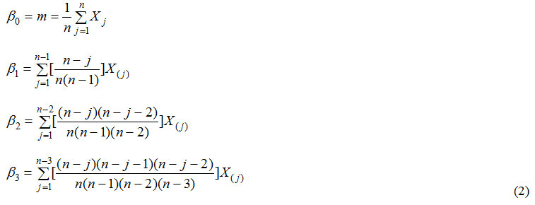
Where x(j) represents the ranked AMS with x(1) being the highest value and x(n) the lowest value, respectively. The first four L-moment are given as follow
 

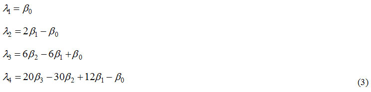
Non-biased sample estimators in the first four L-moments are resulted by the substitution of the PWM sample estimators from Eq. (2) and Eq. (3). The first L-moment λ₀ and the mean value of X are equal. At the end, the L-moment ratios are calculated as:
 

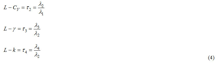
Sample estimates of L-moment ratios are obtained by substituting the L-moments in Eq. (4) with sample L-moments.
 

Heterogeneity Measure

Heterogeneity measure is used for identification of homogeneous regions based on observed and simulated dispersion of L-moments for a group of sites under consideration. This can be computed from¹⁵:
 

Where V = weighted standard deviation of values, , = the mean and standard deviation of N_sim values of , and N_sim = number of simulations.

A region is declared ‘acceptably homogeneous’ if H<1; ‘possibly heterogeneous’ if 1μ_v1 and δ_v1. In addition to the above, two additional measures H1 and H2 based on LCV/LCS and LCS/LCK distances respectively are also considered. The measure H1 indicates whether at-site and regional estimates will be close to each other, while H2 indicates whether the at-site and regional estimates will be in agreement. A large value of H1 usually indicates a large deviation between regional and at-site estimates, whereas a large value of H2 indicates a large deviation between at-site estimates and observed data.

Discordance Measure

Discordance measure, ZDIST, is used to screen out the data from unusual sites, i.e. sites whose at-site sample l-moments are markedly different from other sites and is defined as¹⁶:
 

Where Ui = vector of LCV, LCS and LCK for a site i; S = covariance matrix of V; u^- = mean of vector Ui. A given site is declared discordant if Di≤3. Critical value of  ZDIST defines as¹⁴:
 

Where n is number of At-Sites in studied region.

The neuro-fuzzy structure

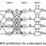
The ANFIS , the multilayer feed-forward network, maps inputs into an output using neural network learning algorithms and fuzzy reasoning. It is certain that a fuzzy interference system (FIS) is implemented in the framework of adaptive neural networks. Fig.1 illustrates the architecture of a typical ANFIS with five layers

Figure 1: A typical ANFIS architecture for a two-input Sugeno model with four Click here to View figure

For simplicity, a typical ANFIS architecture with only two inputs leading to four rules and one output for the first order Sugeno fuzzy model is expressed.^17and18 It is also assumed that each input has two associated membership functions (MFs). It is clear that this architecture can be easily generalized to our preferred dimensions. The detailed algorithm and mathematical background of the hybrid learning algorithm can be found in the Reference.¹⁹

ANFIS-GA Method

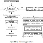
There is a hybrid of canonical real-coded GA, subtractive clustering and ANFIS, designed and finalized for the purpose of producing suitable approximate fuzzy models for the sake of accuracy and parsimony. The primary procedure of modeling is an optimization task executed by GA where both the accuracy and compactness of fuzzy models are the subjects of simultaneous optimization. The whole process of optimization by GA is based on four steps respectively, 1- Fitness assignment 2- Selection 3- Crossover 4- Mutation. Generating a fuzzy model based on subtractive clustering method is completed in the fitness assignment part of GA. The flow chart of modeling procedure is illustrated in Fig.2.

Figure 2: Steps of modeling procedure.  Click here to View figure

Figure 3: Location of wells in Kerman plain.  Click here to View figure

Subtractive clustering method can be used to generate a fuzzy model of TSK in which the number certain rules (i.e. the number of clusters) is determined through radii parameters dedicated into dimensions. These radii are mainly used for the purpose of cluster generation. Each cluster is meant to represent a rule and according to the fact that clustering is completed in multidimensional space, and fuzzy sets for each rule must be achieved. By projecting the center of each cluster in the corresponding dimension, the centers of MFs are obtained. The widths of MFs for a single dimension are obtained on the basis of radius r_a which is particularly considered for that dimension. Therefore, each chromosome in this study acts as radii values encoder for all dimensions inputs and outputs of a fuzzy model. These radii of fuzzy model are then used by subtractive clustering to generate a TSK FIS.

Simulation setup

The population size (PZ) and generation numbers (G) for GA are set to PZ = 100 and G = 50, respectively. The 1-point crossover with the probability of 0.7 is employed. Classical mutation with probability 0.02 is used and selection method is the roulette wheel. Number of epochs and learning rate are set to 100 and 0.2 for ANFIS. Ranges of radii are considered to be in interval 0.^{1, 2}

Results and Discussions

First step to define a homogenous region is choosing the most important clustering parameters. Choosing all important parameters to define a homogeny cluster for a phenomena, increase calculating time and errors, so, choosing the most important parameters would make the calculation simpler, without resulting in any major differences. In this paper, out of effective parameters (time series parameters recorded) more important parameters were selected through regression analysis. Results showed that all of the cations, magnesium ions, sodium percentage, and groundwater level have more effect on salinity as they are shown in the following equations.

EC = 154.446 + 87.852 sumCation   (8)
EC= 68.539 + 83.78 sumCation + 36.094 Mg   (9)
EC= 143.368 + 81.572 sumCation + 43.985 Mg +4.031Na%  (10)
EC = 306.097 + 81.705 sumCation + 38.178 Mg + 5.253 Na% + 1.732 L  (11) 

Where L = groundwater level, the most accurate one is equation No.11 with C.C = 0.97. Moreover, the C.C of each parameter is shown in Table.1

Table 1: Correlation coefficient for different parameters in multiple linear equations  

Therefore, these parameters are used for electrical conductivity in clustering and also input parameters for forecasting. In this paper, with K-Means method and Ward hierarchical, the region was divided into 2, 3, and 4 sectors, respectively. And then, the incompatibility and non-homogeny criteria for the region were defined. For choosing the best clustering mode and optimum number of regions, incompatibility summation of At-Sites, defining the number of incompatible At-Sites with more degree of 1.5, 2 and 3, and also non-homogeny criteria were conducted for each and every region. Results are shown in Table.2

Table 2: Non- homogeny criteria for different scenarios.

Considering Table.2, when all the At-Sites are considered as one region, only the H₁ criteria are homogeny while H₂ and H₃ are non-homogeny. In general, K-mean method includes 4 regions as the priority and Ward, with 4 regions in the next place. Considering 4 homogeny regions for research area, some wells were scattered in the other areas. To solve this problem, all the following, well No3 in region A, well No₁₅ in region B, and well No₂₇ in region D were combined together and then the non-homogeny criteria were computed. Relocation of the wells increased the non-homogeny of region A and B and decreased that of region C. To define the increase of non-homogeny, incompatibility of the wells was investigated and it was observed that well No₁₄ was incompatible. The well was moved to region B and computation was restarted. The results showed decreased incompatibility for well No₁₄. And finally, with moving to region B and re-computation, better results were achieved. Figures below show the final homogeny regions.

Regional Forecasting

First and foremost, for regional forecasting, dimensionless data was computed in each one of the three regions including both selection input data and electrical conductivity. After choosing the best scenario for forecasting, by multiplying average off each well by regional dimensionless data, the dimensionless forecasting data is obtained for each well. Desired periodical statistics are considered on a monthly basis from 2001 to 2013. For analysis, 156 regional dimensionless data were used. In this research, 70 percent of the data was used for teaching, 10 percent for validation, and the remaining 20 percent was used for the testing. Furthermore, for regional forecasting, models constructed with the relation equation are studied. In all models, the momentum training and ANFIS-GA method were used.

Table 3: The best topology of ANFIS-GA model for the study areas

Having observed the results of correlation coefficient and non-homogeny criteria, it is obvious that non-homogeny decreased, the correlation coefficient of the observed data and regional forecasted data decreased as well. The reason is that low non-homogeny means incompatibility of the wells with the other wells in the same region. So, this would be able to reduce forecasting error. After implementing the proposed method (ANFIS-GA) for each region, with multiplying the coefficient of each At-Site for the desired year, by regional forecasting data, electrical conductivity was calculated for each At-Site, and, finally, between the observed and calculated data, the correlation coefficient was calculated. Tables 4 to 6 show the correlation coefficient for each well.

Table 4: The correlation coefficient between observed and predicted data for each well in the area A

Table 5: The correlation coefficient between observed and predicted data for each well in the area B

Table 6: The correlation coefficient between observed and predicted data for each well in the area C

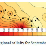
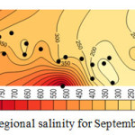
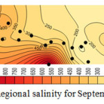
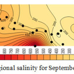
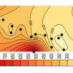
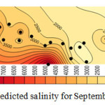
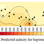
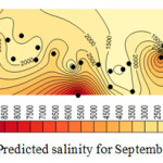
Considering the results shown in tables 4, 5, and 6 the wells No₃, No₁₄, No₁₅ and No₂₇ which were moved before, have the least correlation coefficient. Better correlation coefficients are associated with the wells with salinity levels close to that of the regional average. Thus, it follows that regional analysis can forecast with high precision, in case of selection of wells and internal At-Sites. Figures 4, 5, 6, and 7 show forecasting and regional salinity.

Figure 4: Regional salinity for September 2001   Click here to View figure

Figure 5: Regional salinity for September 2007   Click here to View figure

Figure 6: Regional salinity for September 2011   Click here to View figure

Figure 6: Regional salinity for September 2013   Click here to View figure

Figure 7  Click here to View figure

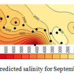
The figures 8, 9, 10, and 11 show the salinity of each at-site which is obtained from multiplying the average at-site by regional forecasting data. The horizontal axis is represented EC concentration as it is illustrated in figures 8 to 11 the concentration of EC increase from 8000 micromohs in 2001 to 10000 micromohs in 2013.
 

Figure 8: Predicted salinity for September 2001 Click here to View figure

Figure 9: Predicted salinity for September 2007   Click here to View figure

Figure 10: Predicted salinity for September 2011   Click here to View figure

Figure 11: Predicted salinity for September 2013   Click here to View figure

At-Site forecasting

For forecasting the salinity of our 34 wells, similar to the regional method, the proposed method ANFIS-GA is applied to each well. For this purpose, the correlation coefficient between the observed data and forecasted data was obtained. After choosing the appropriate model, the forecasting started. Review of the results suggests that the salinity of groundwater for the study area increased during the past years. And also it's clear that ANFIS-GA is capable of forecasting acceptable groundwater salinity.

Comparison of At-Site and regional forecasting

Priority of regional or At-Site analysis for each studied well of Kerman plain was revealed through the method of correlation of coefficient, and then inserted into Table 7.
 

Table 7: Correlation coefficient for best structures at different Wells

According to the results mentioned above, 21 wells with regional analysis and 13 wells with At-Site analysis method maintain good accuracy. The investigation shows that for wells, for which regional analysis shows lower accuracy in comparison to At-Site analysis, the average is above regional average (wells No₁ ,No₅, No₉, No₁₅, No₁₉ and No₂₂) or below regional average (wells No₂₃, No₂₈ and No₃₃). The rate of incompatibility for these wells is higher than the other regional homogenous wells. Region A has the most priority in At-Site analysis followed by C and D. As a result, the most important regions for analysis are the non-homogenous regions. As a result, in case of proper selection of the at-sites in a homogeneous region and low at-sites incompatibility as well as non-homogeneity criterion, regional analysis is preferable to at-site analysis.

Conclusion

According to regression analysis, sum of cat-ions, magnesium ions, percentage of sodium, and groundwater table are the most effective on salinity. Moreover, for defining the number of homogeny clusters, generally, K-Means method, with 4 regions is the first and Ward with 4 regions is the second suitable selection. As the non-homogeny criteria decreased, correlation coefficient between the observed data and regional forecasted data reduced as well. The largest correlation coefficient was associated to the wells with close salinity to the regional average. In case of precise selection of the wells and At-Sites inside the region, the regional analysis can forecast with high accuracy. The most important regions for analysis are the non-homogenous regions. Moreover the ANFIS-GA model analysis showed an increase in the compactness and accuracy of the mentioned model during the testing stage. Our proposed method aiming to provide us with the best and effective composition of structure in the ANFIS model trade off rise and fall between the accuracy and the number of certain parameters. The maintained results are to show a new hybrid algorithm providing both accuracy and complexity for a Neuro-Fuzzy model.

References
 

1. Shu, C., Ouarda, T.B.M.J. (2008). Regional flood frequency analysis at engaged sites using the adaptive neuro-fuzzy inference system. Journal of Hydrology., V.349, PP.31-43.
   CrossRef
2. Furst, j., Bichler, A. and Konecny, F. (2014). Regional Frequency Analysis of Extreme Groundwater Level. Journal of Grounwater, Jonwielly.
3. Jalalkamali, Amir.,Sedghi, Hossein., Manshouri, Mohammad .(2011)., Monthly groundwater level prediction using ANN and neuro-fuzzy models: a case study on Kerman plain, Iran, Journal of hydroinformatics (13.4) 867-876.
4. Adamowski, Jan., Fung Chan, Hiu. (2011)., A wavelet neural network conjunction model for groundwater level forecasting, Journal of Hydrology (407) 28–40.
   CrossRef
5. Lohani, AK., Krishan, G. (2015) Application of artificial neural network for groundwater level simulation in Amritsar and Gurdaspur districts of Punjab, India. Journal of Earth Science and Climate Change 6:274.
6. Samson,M., Swaminathan, G., Venkat Kumar, N.(2010)., Assessing groundwater quality for portability using a Fuzzy logic and GIS – a case study of Tiruchirappalli city – India, Computer Modeling and New Technologies., Vol.14, No.2, 58–68.
7. Jalalkamali, Amir. (2015)., Using of hybrid fuzzy models to predict spatiotemporal groundwater quality parameters, Earth Science Informatics, DOI 10.1007/s12145-015-0222-6.
   CrossRef
8. Jalalkamali, Amir. Moradi, Mehdi., Moradi, Nasrin. (2015)., Application of several artificial intelligence models and ARIMAX model for forecasting drought using the Standardized Precipitation Index, International Journal of Environmental Science and Technology, Volume 12, Issue 4, pp 1201-1210.
   CrossRef
9. Lohani, AK., Krishan, G. (2015)., Groundwater Level Simulation Using Artificial Neural Network in Southeast, Punjab, India, Journal of Geology & Geophysics 4: 206.
10. Seyam, Mohammed.,Mogheir, Yunes. (2011). A NEW APPROACH FOR GROUNDWATER QUALITY MANAGEMENT, the Islamic University Journal (Series of Natural Studies and Engineering), Vol.19, No.1, pp 157-177.
11. Nowjavan, M.R. (2015). Analysis of Water Resources and Its Relation to Geological Structure in Arid and Semiarid Areas (Case Study: Plains of Kerman Province), Vol 6 No, pp 720-727.
12. Hosking, J.R.M. (1990). L-moments: Analysis and estimation of distributions using linear combinations of order statistics: J.R. Stat. Soc., Ser. B, 52, 105-124.
13. Greenwood, J.A., Landwehr, J.M., Matalas, N.C., and Wallis, J.R. (1979). Probability weighted moments: Definition and relation to parameters of several distributions expressable in inverse form. Water Resources Research, 15(5), 1049-1054.
    CrossRef
14. Hosking, J. R. M., & Wallis, J. R. (1997). Regional Frequency Analysis: An Approach Based on L-Moments. Cambridge Univ. Press, New York.
    CrossRef
15. Kjeldsen, T. R., Jones, D. A. (2006). Prediction uncertainty in a median-based index flood method using L- moments. Water Resources Research, V. 42.
    CrossRef
16. Rostami, R., & Rahnama, M. B. (2007). Halil-river Basin regional flood frequency analysis based on l-moment approach. International journal of agriculture researches, USA, Newyork.
17. Sugeno, (1985)Industrial applications of fuzzy control. Elsevier Science Pub.Co.
18. Wang,YM.,Elhag, T. (2008) An adaptive neuro-fuzzy inference system for bridge risk assessment. Expert Systems with Applications 34(4): 3099-3106.
    CrossRef
19. Jang JSR. (1993) ANFIS: Adaptive-network-based fuzzy inference systems, IEEE Transactions on Systems Man and Cybernetics, 23 (3), pp 665–685.
    CrossRef