Stream Flow Modeling for Ranganadi Hydropower Project in India Considering Climate Change
Manti Patil1 *
1
Department of Civil Engineering,
Oriental University,
Indore,
MP
India
http://dx.doi.org/10.12944/CWE.11.3.19
The Stream-flow is key component of hydro power project regulation. The present study has been conducted to identify the impact of climate change on stream flow of Ranganadi River, a sub-set of Brahmaputra basin situated at north-East region of India, which receives more rainfall as compare to other parts of India The three GCM model viz.HadCM3, CGCM2 and GFDL monthly data with A2 scenario have been choose for Downscaling by advanced neural technique (Artificial Neural Network).The prediction result show as an positive increasing trend up to 2040 for Ranganadi River. This will create the flood problem but capacity of hydroelectricity generation will be increase.
Copy the following to cite this article:
Patil M. Stream Flow Modeling for Ranganadi Hydropower Project in India Considering Climate Change. Curr World Environ 2016;11(3). DOI:http://dx.doi.org/10.12944/CWE.11.3.19
Copy the following to cite this URL:
Patil M. Stream Flow Modeling for Ranganadi Hydropower Project in India Considering Climate Change. Curr World Environ 2016;11(3). Available from: http://www.cwejournal.org/?p=16581
Download article (pdf) Citation Manager Publish History
Introduction
Forecasting of daily, monthly or longer time interval stream flow is most important for the reliable operation of a water resources system. Reliable Stream flow forecast can allocate water efficiently for competing water users like hydropower generation, agricultural and domestic for maintenance of environmental flows. Various studies have been performed for impacts assessment of climate change on hydropower projects.1,2 The possible impact can be categorized into three head that is: (a) the available discharge of water may change since; hydrology is usually related to the local weather condition, such as temperature and precipitation in the catchment area.8 This will influence on economic and financial variability of hydropower project. Due to seasonally change if the flow of water changes, different power generating operation like peak versus base load would be possible using reservoir.(b) Expected increase in climate variability may trigger extreme climate events floods and droughts. Hydrological model indicates the great risk of Bangladeshi suffering from extreme floods, which are lead sustainable increase in peak discharge in the three regional rivers, Ganga Brahmaputra and Meghna. (c) Changing the hydrology and possible extreme events must necessarily impact on sediment risk and measures. Hydropower project may suffer great exposure to turbine erosion due to sediment along other factors such as changed composition of water.13 There are several modeling techniques have been used worldwide researcher for down scaling and climate assessment like SVM, ANN,2 one of them artificial neural networks has been effectively used in modeling various water related processes. The artificial neural network is inspired by functioning human brain. It has experienced a vast revitalization due to the development of more advanced algorithms and with the emergence of more powerful computers. Mathematically, an ANN is often viewed as a universal approximate. The ability to identify the relationship from given pattern makes it suitable for ANNs to analysis and solve large scale complex problem like pattern recognization, nonlinear modeling, and classification.The utility of feed forward neural network model for stream flow forecasting was better than conventional model like regression analysis or linear model.3 Developed ANN model for Mountain watershed and concluded that the selection of input variables, defined the strength of model learning process during calibration. Moreover, the Results showed that that spring and summer monthly stream flow can be adequately represented improving the results of calculations obtained using the other methods.5 Similar finding have been recognized by6 for of the Hemavathi river basin. The trained network is used for both single step and multiple step forecasting. It was concluded that the recursive neural network perform well than FFN for forecasting monthly river flows in both single time step and multiple time steps.
As has been discussed above climate change will change the occurrence and distribution of the water scope. As such, the main focus of this project is to see the possible impact of climate change on the future flow scenario of the Ranganadi River as well as the subsequent impact on the hydropower generation.14 Ranganadi is one of the tributaries of the Brahmaputra River. For the prediction of future flow, an artificial neural network model is then developed for downscale the GCM data. The ANN downscaling model is then used to predict the future stream flow of the river.7 View on this the specific objective are fallowed: (A) to see the possible impact of climate change on stream flow of Ranganadi River. (B) Impact on Ranganadi hydropower generation.
Study Area
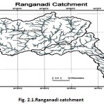
The study area Ranganadi River about 1749 sq.km is one of the major tributaries of the Brahmaputra River. It originates from the Tapo mountain ranges in Arunachal Pradesh. The study area is located between 94â°02’34” E longitude and 27â°14’01” N latitude in the Brahmaputra River basin of India as depicted in Fig 2.1. The flow of the Ranganadi River is regulated by the Ranganadi 405 MW Hydroelectric project dam. The Ranganadi dam is a concrete-gravity dam on the Ranganadi River in Arunachal Pradesh, which serves a run of river scheme. The dam is intended for hydroelectric purpose and is part of stage 1 of the Ranganadi hydroelectric project and supports the 405 MW Dikrong power house at 27Ëš15’27” N 93Ëš47’32”E.
 |
|
Data Used
Stream Flow Data
For the present study, as per availability, 20 years monthly flow data used in two different intervals from 1972-1982 and 2001-2009.
Gcm Data
General Circulation Model (GCM) is a mathematical tool of the general circulation ofocean or the planetary atmosphere and simulates the time series of climate variability globally accounting for effects of greenhouse gases and environment.5 GCM is also known as the global climatic model. In this study, three GCM have used (HadCM3 CGCM2 and GFDL) for impact assessment. HadCM3 stands for Hadley Centre Coupled Model version 3. This model does not require flux adjustment. In this model, spatial resolution for CGCM3 is roughly 2.5 degree of latitude and 3.75 degrees of longitude.CGCM2 stands for second generation of Couple Global Climate Model. Atmospheric Global Climate Model and Oceanic Global Climatic Model are the two main component of this model. Spatial resolution of CGCM2 is roughly 3.75 degrees latitude and longitude and 31 levels in vertical. In OGCM2 spatial resolution 1.85 degrees and vertical levels equal to 29. The Geophysical Fluid Dynamic Laboratory (GFDL) is coupled atmospheric-oceanic general circulation model. The model has been shown to produce a very faithful simulation of the observed seasonal cycle and year to year variability in the tropical Atlantic. The spatial resolution is 2.25 degree latitude and 3.75 degree longitude.
 |
|
Material and Methods
Downscaling is a technique that takes the output from the model and adds the information at smaller scales. Global climate models (GCMS) are run at coarser spatial resolution which cannot be used directly in the local impact studies due to cloud cover and other effects. To overcome this problem, down scaling methods are generating to obtain local-scale surface weather parameters from regional-scale atmospheric variables which are provided by GCMs.15 Neural network is one of the tools used for methodological analysis of hydrological forecasting.16 It can be thought of as a computational pattern that involves searching and matching procedures, which permits forecasting without an intimate knowledge of the physical process. The neural network seeks the relationship between input and output data and then creates its own equations to match the pattern in an iterative manner.17 In this study the best model has been decided by varying the different algorithms and varying the number of hidden neuron from 1 to 15 with various combination of learning rate from 0.01 to 0.9 and momentum factor from 0.01 to 0.9. Forecasting has been followed in three clearly separate stages. They are training mode, validation and testing phase. In training mode, the output is linked to as many of the input nodes as desired and pattern is defined. The network is adjusted according to this error. The validation dataset is used at this stage to ensure the model is not over trained. In testing phase, the model is tested using the dataset that was not used in training.
The data is normalized before entering into the neural network. Due to the nature of the algorithm, large values slowdown training process. This is because of the gradient of the sigmoid function at extreme values approximate to zero. Mean and Standard Deviation (mapstd), an approach for scaling the network inputs and targets so as to minimize the standard deviation and mean of the training set. The mapstd function normalizes the inputs and targets so that they will have zero mean and unity standard deviation. The original network inputs and targets are given in matrices and. They effectively work a part of the network, just like the biases and network weights. After this, the outputs are converted back into the same units.11
Selection of Predictors
Pearson correlation is used for selection of predictor Pearson correlation is a simple correlation between predictor and predictant. In the correlation test, “0” represent weak correlation whereas “1” represents strong correlation.
Table 4.1 shows the correlation between observed stream flow data and GCM simulated data
|
S.NO. |
HadCM3 Predictors |
Correlation of HadCM3 with observed runoff at point 1 |
|
1 |
Sea level pressure |
0.2396 |
|
2 |
Relative humidity |
-0.0459 |
|
3 |
Relative humidity@200 hpa |
0.0789 |
|
4 |
Relative humidity@500 hpa |
0.2088 |
|
5 |
Geo-potential height @200 hpa |
0.0186 |
|
6 |
Geo-potential height @500 hpa |
0.0088 |
|
7 |
Geo-potential height @850 hpa |
-0.3064 |
|
8 |
short wave radiation flux |
0.2471 |
|
9 |
Humidity mixing ratio |
0.1030 |
|
10 |
Temperature |
0.1971 |
|
11 |
Temperature@850 hpa |
0.2147 |
|
12 |
Maximum temperature |
0.2053 |
|
13 |
Minimum temperature |
0.1688 |
According to this table, the predictor that shows the best correlation value will be used in the next step.
Table 4.2: List of selected predictors
|
Location |
Predictands |
Predictors |
|
Point |
runoff |
Mean sea level pressure Surface air temperature Air temperature@850 hpa Relative humidity@500 hpa Short wave radiation |
Table 4.3: Correlation between CGCM2 and observed
|
S.NO. |
CGCM2 Predictors |
Correlation of CGCM2 with observed runoff |
|
1 |
Sea level pressure |
-0.2133 |
|
2 |
U componant of velocity |
0.0129 |
|
3 |
Dew point depression |
0.1643 |
|
4 |
Temperature |
0.1672 |
|
5 |
Geo-potential height |
- 0.0227 |
|
6 |
Geo-potential height @500 hpa |
-0.221 |
|
7 |
Stream function |
-0.0485 |
|
8 |
short wave radiation flux |
-0.2790 |
|
9 |
Total precipitation |
0.1760 |
|
10 |
Maximum temperature |
0.1686 |
|
11 |
Minimum temperature |
0.1657 |
Table 4.4: List of selected predictors
|
Location |
Predictands |
Predictors |
|
Point |
Runoff |
Mean sea level pressure |
|
Surface air temperature |
||
|
Maxi. temperature |
||
|
Mini. Temperature |
||
|
Total precipitation |
Table 4.5: Correlation between GFDL and observed data
|
S.NO. |
GFDL Predictors |
Correlation of GFDL with observed runoff |
|
1 |
Shoret wave |
-0.1991 |
|
2 |
Perceptible water |
0.0193 |
|
3 |
Total precipitation |
-0.0256 |
|
4 |
Pressure |
0.0220 |
|
5 |
Temperature |
0.0701 |
|
6 |
Dew point depression |
0.1585 |
|
7 |
U wind |
-0.991 |
|
8 |
V wind |
-0.0339 |
Table 4.6: List of selected predictors
|
Location |
Predictands |
Predictors |
|
Point
|
Runoff |
Total precipitation Temperature Dew point depression Perceptible water |
Performance Indicator
For goodness of fit the correlation coefficient (R) and Mean square error has been used by ANN model and Microsoft Excel.
Results
This chapter deal with the results obtained from ANN based stream flow modeling. An attempt has been made to develop ANN model for prediction of stream flow of Ranganadi River. Mean and standard deviation (mapstd) function was used for scaling all input and target data using MATLAB .In this study, we have follow up three GCM models for providing the input parameters to ANN model based downscaling method, HadCM3 CGCM2 and GFDL model were used for prediction of stream flow of Ranganadi River. With each one of the GCM models, we have varied the seven different algorithms for achiving the best ANN model. The ANN model takes into consideration adaptive system with different layer of hidden neurons, so we have also varied the no of neuron with each algorithm and each model.
Evaluation of Best Optimization Algorithms and Optimum Number of Hidden Neurons of the ANN Model for HadCM3 GCM
Initially, the single GCM point available near the study area is used for prediction the future flow of the river Ranganadi. The Table 5.1 shows the comparative study with levenberg-marquardt algorithm.6 It can be seen that MSE is 0.064 when number of hidden neurons is 8. According to that the table 5.2 shown the MSE 0.085 when number of hidden neurons is 5 with batch gradient descent algorithm. The table 5.3 shows that the minimum MSE occurs when number of hidden neurons is 8 and its value is 0.904 with variable learning rate algorithm. The Resilient propagation algorithm shows minimum MSE value of 0.095 for number of hidden neurons equal to 10, as mentioned in table 5.4. The scale conjugate gradient algorithm shows MSE value of 0.102 in table 5.5 when number of hidden neurons is 8. The table 5.6 shows the minimum MSE of 0.089 when number of hidden neurons is 5 with quasi Newton algorithm. Quasi Newton one step secant algorithm shows the minimum MSE as 0.077 for number of neurons equal to 11. From the table5.1, it can be seen that MSE is minimum when the number of hidden neurons is 8 with levenberg-marquardt algorithm. This study suggests levenberg-marquardt algorithm is the best algorithm to train the network in this case.
Table 5.1:- Performance of neural network with levenberg-marquardt algorithm
|
No of Neuron(trainlm) |
Training |
Validation |
Testing |
All |
M S E |
|
R |
|||||
|
N3 |
0.7766 |
0.58 |
0.8173 |
0.716 |
0.057 |
|
N4 |
0.7674 |
0.7041 |
0.6438 |
0.6984 |
0.08 |
|
N5 |
0.7629 |
0.6065 |
0.8437 |
0.7139 |
0.065 |
|
N6 |
0.7916 |
0.5957 |
0.6157 |
0.7081 |
0.1 |
|
N7 |
0.877 |
0.5608 |
0.5756 |
0.769 |
0.11 |
|
N8 |
0.7115 |
0.789 |
0.702 |
0.695 |
0.064 |
|
N10 |
0.943 |
0.4894 |
0.5056 |
0.8069 |
0.128 |
|
N11 |
0.969 |
0.4918 |
0.5713 |
0.8556 |
0.084 |
|
N12 |
0.9267 |
0.6067 |
0.5993 |
0.8161 |
0.098 |
|
N13 |
0.9618 |
0.581 |
0.6219 |
0.8777 |
0.063 |
From the table 5.1 it can be seen that learning function ‘trainlm’ is the best as per the training algorithms are concerned. Selection of optimum numbers of neurons is an essential part of ANN model development. The trainlm algorithm with 50% data is for training and 50% for validation and testing, has been evaluated for optimum number of neurons. Number of hidden neurons has been varied from 1-15. The performance of ANN model with N=8 is shown in table 5.1. It is seen that the MSE is minimum, with a value of 0.064, with training =0.711, validation =0.789 and testing value is 0.7016.
 |
|
 |
|
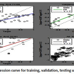
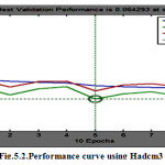
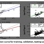
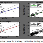
The fig 5.1 shows the Regression curve indicate training, validation, testing, and all R value, where data is varying between the training, validation, testing line and best fit line. Our purpose is to set the data along the best fit line so that we achieve the best regression value. In the fig 5.1, validation data is very close to the best fit line. The performance curve in fig 5.2 shows the MSE for training, validation and testing. For epoch 5, the fig 5.2 clearly shows that the validation line is very close to the best fit line. If these two lines overlap, it means that the MSE value has been minimized.
After this, the average value of five HadCM3 points which are in and around study area is taken and the regression and MSE value are obtained for prediction of stream flow. The average value of five points gave optimum result for training and validation but performance MSE value is not acceptable as shown in table 5.9
Table 5.2:- Performance of ANN at average of five points with different number of neurons
|
No of Neuron |
Training |
Validation |
Testing |
All |
M S E |
|
(trainlm) |
R |
||||
|
N3 |
0.773 |
0.490 |
0.728 |
0.696 |
0.100 |
|
N4 |
0.924 |
0.655 |
0.630 |
0.756 |
0.120 |
|
N5 |
0.827 |
0.407 |
0.779 |
0.665 |
0.200 |
|
N6 |
0.815 |
0.438 |
0.662 |
0.628 |
0.103 |
|
N7 |
0.958 |
0.652 |
0.730 |
0.595 |
0.129 |
|
N8 |
0.945 |
0.653 |
0.703 |
0.740 |
0.101 |
|
N9 |
0.935 |
0.586 |
0.565 |
0.515 |
0.160 |
|
N11 |
0.956 |
0.498 |
0.712 |
0.630 |
0.310 |
|
N12 |
0.935 |
0.553 |
0.209 |
0.382 |
0.150 |
Evaluation of Best Optimization Algorithms and Optimum Number of Hidden Neurons of the ANN Model for CGCM2 GCM
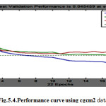
The study is also carried out considering CGCM2 data in this case also, the point data available near to the study area is considered as the input of the ANN model. Table 5.9 shows the result with levenberg marquardt algorithm, the minimum MSE being 0.045 with number of neurons as 6. Levenberg marquardt algorithm shows the best minimum MSE value as compared to other algorithms with CGCM2 model. Table below shows the results of each algorithm.
Table 5.3: Performance of ANN with CGCM2 data using levenberg-marquardt algorithm
|
No of Neuron |
Training |
Validation |
Testing |
All |
M S E |
|
(trainlm) |
R |
||||
|
N3 |
0.7584 |
0.65993 |
0.555 |
0.6843 |
0.067 |
|
N4 |
0.7705 |
0.69935 |
0.6485 |
0.7186 |
0.062 |
|
N5 |
0.7902 |
0.6195 |
0.4925 |
0.6718 |
0.07 |
|
N6 |
0.8762 |
0.7712 |
0.69 |
0.8 |
0.045 |
|
N7 |
0.8133 |
0.6725 |
0.622 |
0.7134 |
0.068 |
|
N8 |
0.8802 |
0.7097 |
0.5997 |
0.7385 |
0.07 |
|
N9 |
0.7994 |
0.6887 |
0.5816 |
0.7118 |
0.063 |
|
N10 |
0.7396 |
0.5528 |
0.4584 |
0.6303 |
0.077 |
|
N11 |
0.81384 |
0.6773 |
0.4456 |
0.6892 |
0.066 |
|
N12 |
0.8229 |
0.468 |
0.3953 |
0.6029 |
0.089 |
|
N13 |
0.8028 |
0.5401 |
0.5281 |
0.6388 |
0.066 |
|
N14 |
0.9019 |
0.6534 |
0.3685 |
0.6973 |
0.086 |
 |
|
 |
|
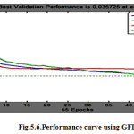
Finally, we have followed up the GFDL model parameters as inputs in ANN model .In the table below, the results of GFDL have been shows and precise result of each algorithm has been highlighted. Levenberg-marquardt algorithm shows training= 0.8220, validation = 0.8298, testing= 0.7299, over all R= 0.7973 with the MSE= 0.035 which is the minimum MSE out of all three models and seven algorithms. After the use of these three GCM models the results focus that the GFDL model is best for stream flow prediction of this area.
Table 5.4: Performance of neural network with GFDL data using Levenberg-Marquardt algorithm
|
No of Neuron |
Training |
Validation |
Testing |
All |
M S E |
|
(trainlm) |
R |
||||
|
N3 |
0.819 |
0.7134 |
0.6621 |
0.7477 |
0.049 |
|
N4 |
0.888 |
0.69277 |
0.6971 |
0.7844 |
0.047 |
|
N5 |
0.7679 |
0.7099 |
0.572 |
0.6915 |
0.057 |
|
N6 |
0.8655 |
0.7312 |
0.6719 |
0.7676 |
0.048 |
|
N7 |
0.9253 |
0.7722 |
0.7764 |
0.843 |
0.034 |
|
N8 |
0.8825 |
0.6563 |
0.7736 |
0.7966 |
0.054 |
|
N9 |
0.8911 |
0.5797 |
0.7585 |
0.7738 |
0.065 |
|
N10 |
0.822 |
0.8298 |
0.73 |
0.797 |
0.036 |
|
N11 |
0.8622 |
0.4004 |
0.5978 |
0.638 |
0.072 |
|
N12 |
0.7836 |
0.5082 |
0.5334 |
0.6449 |
0.067 |
 |
|
 |
|
Simulation of future runoff of river Ranganadi
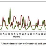
The above analysis reveals that the best GCM out of the three GCM model considered in the study is the GFDL GCM model. As such the GFDL model is used in the study to predict the future flow scenario of the river. The ANN model trained With Levenberg-Marquardtalgorithm and also with hidden neuron of 10 is used for predicting the future discharge of the river. Fig 5.7 prediction plot indicates increasing trend of stream flow.
 |
|
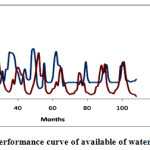
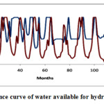
As discussed earlier, a hydropower project is exists on the river Ranganadi. Approximately 414.72 mcm water is necessary for proper production of hydropower at its full capacity. The storage capacity of thr reservoir is around 15 mcm. Based on increasing trend of stream flow in future a simulation is carried out to estimate the volume of water that will be available for electricity generation. If available water is greater than or equal to 414.72mcm, then there will not be any shortage of water for power production in future. If monthly available water is less than 414.72 mcm, then it will not be possible to run the power house to its full capacity. Fig 5.8 indicates the available water per month for the base line period and also shows the available water for future period. It shows that in the future, amount of water as compare to present except for few months.
 |
|
Fig 5.8 shows available amount of water for hydropower generation at present and future. It can be seen that in water available in future will be more in comparison to the baseline period. As a result of increasing flow, the electricity generation by the power project will be more. It may be noted that this study is carried out considering monthly flow data of river. The project is run-of- river project with very less storage capacity. As such, the actual availability of water for power production on daily basis may be different and may not more power in future. However, for the bigger project with large storage capacity, the future power production may be more than the baseline period.
 |
|
Discussion
Climate change is a hydrological phenomena and its variation is occurs in nature. So that I have consider three model and taking inputs which moving average of 5 years interval to minimize the variation. In this study, we have follow up three GCM models for providing the input parameters to ANN model based downscaling method, HadCM3 CGCM2 and GFDL model were used for prediction of stream flow of Ranganadi River. Input parameter has selected with results of best correlation between simulated and observed data. The basic ANN was optimized in terms of training algorithm, number of neurons in hidden layer and changes the various combinations of learning rate and momentum coefficient. By using various combinations of algorithm and number of neurons used to minimize the performance error, the best result was obtained for levenberg-marquardt algorithm with number of hidden neuron as 10. Simulation work has done by best optimized model. Fig 5.7 prediction plots indicate that the scenario of stream flow at 2040 will be in increasing trend.
Conclusion
In this study, the possible future stream flow has been predicted for Ranganadi River. The prediction has done by downscaling using artificial neural network. The basic ANN was optimized in terms of training algorithm, number of neurons in hidden layer and changes the various combinations of learning rate and momentum coefficient. By using various combinations of algorithm and number of neurons used to minimize the performance error, the best result was obtained for levenberg-marquardt algorithm with number of hidden neuron as 10. Simulation work has done according to hydropower project which exists on the river Ranganadi. Approximately 414.72 mcm(data collected from power house at Arunachal Pradesh) water is necessary for proper production of hydropower at its full capacity. The storage capacity of the reservoir is around 15 mcm. Fig 5.7 prediction plots indicate that the scenario of stream flow at 2040 will be in increasing trend. Based on increasing trend of stream flow in future a simulation is carried out to estimate the volume of water that will be available for electricity generation. If available water is greater than or equal to 414.72mcm, then there will not be any shortage of water for power production in future. If monthly available water is less than 414.72 mcm, then it will not be possible to run the power house to its full capacity. Fig 5.8 indicates the available water per month for the base line period and also shows the available water for future period. It shows that in the future, much more amount of water as compare to present except for few months. So, electricity generation will higher and we can allocate remains amount of water for different purposes.
References
- Chang, J. and Wang,Y. Impact of Climate Change and Human Activity on Runoff in Weich River basin China. Elsevier Vol. 380-381 (2015)
- Kisi, O.[Stream flow Forecasting using different Artificial Neural Network algorithms . Journal of hydrologic Engineering (ASCE) 1084-0699(2007)12:5(532) (2007).
- Zealand, C. M., Burn, D. H. and Simonovic, S. P. Short term Stream flow Forecasting using Artificial Neural Networks. Journal of Hydrology. 214, 32–48(1999).
CrossRef - Kumar, D. and Bhattacharya, R. K.,. Distributed Rainfall Runoff Modeling . International journal of Earth Science and Engineering. Volume 04, No 06 SPL, 270-275 (2011).
- Intergovernmental Panel on Climate Change Climate Change: Impacts, Adaption and Vulnerability . Contribution of working group to the Fourth Assessment report of Intergovernmental Panel on Climate Change. Cambridge, UK: IPCC. ( 2007)
- Adam, P.P., Jaroslaw, J., N. Optimizing Neural Networks for River flow Forecasting - Evolutionary Computation methods versus the Levenberg-Marquardt apporch 407(2011) 12-27. ( 2011)
- Ahmed, J. A., Sarma, AK.. Artificial Neural Network model for Synthetic Stream flow generation. Water resources Management 21(6): 1015-1029. (2007)
CrossRef - Estimation of Global Climate Change Impacts on Hydropower projects: Application in India Sri Lanka and Vietnam (FEU)
- Imrie, C. E., Durucan, S.and Korre, A.River flow prediction using artificial neural network: generalization beyond the calibration range. Journal of Hydrology 223(2000)138-153.( 2000)
- Mujumdar, P. P.,“Implications of climate change for sustainable water resources managemen t in India”, Physics and Chemistry of the Earth, 33, pp. 354-358. (2008)
CrossRef - Karunanithi, N., Grenney, W. J., Whitley, D. and Bovee, K.. Neural networks for river flow prediction . ASCE J. Cmp. Civil Eng. 8(2), 201–220.( 1994)
CrossRef - Kumar D.N., Raju S.K. and Sathish T. River flow Forecasting using Recurrent Neural Networks. Water Resources Management 18:143-161. (2004).
CrossRef - Raghuwanshi, N.S., Singh, R. and Reddy, L.S.,. Runoff and Sediment yield Modeling using Artificial Neural Networks:Upper Siwane River, India. J Hydraulic Eng ASCE.,11(1): 71–79. ( 2006)
- Subimal Ghosh, Deepshree Raje and Mujumdar P.P.,,“Mahanadi Stream Flow : Climate Change Impact Assessment and adaptive strategies”, Current Science, Vol. 98, No. 8, pp.1084-1091. ( 2010)
- Wikipedia, the free encyclopedia “Global climate model ” assessments of climate parameter. http://en.wikipedia.org/wiki/global
- Yonas, B. Dibike, Paulin, Coulibaly, “Hydrologic Impact of Climate Change in the Saguenay Watershed comparison of Downscaling methods and Hydrologic models”, Journal of Hydrology,Vol. 307, pp.145–163. ( 2004).
- Ray, R.M., and Sarma AK. Importance of Input parameter selection for Synthetic Stream Flow generation of different time step using ANN techniques. Department of civil Engineering. IIT Guwahati. (2007)


