Current World Environment

Introduction

After precipitation, the temperature is found to be an essential meteorological parameter of climate. It is also considered as a good indicator to understand the global climate as it signifies the exchange of energy process over the surface of the earth with proper accuracy (Shukla et al., 2015 and Jhajharia & Singh., 2011). In 2007, Intergovernmental Panel on Climate Change (IPCC) stated the growing tendencies of temperature is about 0.74°C of mean temperature in past 100 years from 1906 to 2005 in several areas of the world with respect to space and time. Reiter et al. (2012) observed an increase in temperature in the Upper Danube basin with a rise of 0.8°C /decade during summer. Even in spring and winter temperatures have also shown a constant increase. In the past 500 years, the month wise surface temperature in Europe has never been as warmer as is growing in 21^st century (Luterbacher et al., 2004). In past 53 years, the annual average temperature in Canada has increased by 1.2°C (Vincent et al., 2007). According to IPCC 2007, upwards trends have also been detected across the 7 subregions of Asia. In Russia the rise in mean yearly temperature is observed to be 2 to 3°C (Savelieva et al., 2000; Peterson et al., 2002), 0.7°C in Northwest part of China (Shi et al., 2002), 1.0°C in Japan (Ichikawa, 2004), 1.8°C in main towns of Mongolia (Batima et al., 2005).

A few studies have been carried out in India as well on temperature changes and their alliance with climate change. A temporal and spatial change of annual and seasonal temperature was conducted in India by researchers including Shukla, R., and Khare, D., (2013), Mishra et al., (2013), Darshana et al., (2012), Revadekar et al., (2011), Indrani Pal et al., (2009), Jhajharia et al., (2009), Bhutiyani et al., (2007).   

Darshana et al., (2012) reported that the average annual precipitation variation was (694 mm, Westnimar) to (1416 mm, Mandla). The annual precipitation showed a maximum reduction (-11.99%, Balaghat) and minimum (-8.52%, Shahdol) district. For annual precipitation year, 1978 was found to be the most probable year of change. Alteration in mean percentage of 1901-1978 over the period of 1979-2002 has also been found showing the decrease in precipitation virtually in whole stations. Also in 102 years in Madhya Pradesh, the decrease in annual precipitation was 2.59%. During the period 1901-1978 west part of MP was observed with more rise in yearly precipitation as compared to east part of MP.

Revadekar et al., (2011) conducted the observational analysis by taking 121 stations spread all over India showed that widespread warming through an increase in intensity and occurrence of warm events and also by a decrease in the occurrence of cold actions.   

Indrani Pal et al., (2009) reported that the long period trends in variations of the highest and lowest values of monthly temperatures and their effects on seasonal fluxes in various regions in India. The trends magnitude and statistical significance were determined by least square regression techniques and the varia­tions were regulated by the relevant coefficient of variations. The outcomes is that the monthly maximum temperature raised, though unevenly, over the 20^th century. The minimum temperature changes were more variable than maximum, both temporally and spatially, with lesser significance results. This study showed good pointers of Indian climate changeability over the 20^th century.

Jhajharia et al., (2009) examine the year wise average temperature variation (5 to 30°C) and the average relative humidity between (70 to 85%) for the many part in north-east India. In 2010, (Jhajharia and Singh) finds the decreasing trends in Diurnal Air Temperature (DTR) at 4 stations in north-east for every timescales. Instead, the DTR trends were significant at annual, seasonal (pre-monsoon and monsoon), & monthly (May, June, August, September, and November). Major rising trends in DTR are detected at 3 stations in october month as well as in post-monsoon & monsoon seasons. The 4 sites showed significant rising trends for T_mean at post-monsoon seasons. For post-monsoon, the T_max and T_min are found to be more than monsoon in the seasonal cycle. Significant declining trends during sunshine hours were observed on the basis of winter, pre-monsoon and monthly timescales.

Bhutiyani et al. (2007) demonstrated that the existence of possible variation between the precipitation and temperature in the late-1960s century. However, post-1970, these connections appear to have grown weaker. This points out the presence of other climatic factors (rise of greenhouse gasses etc.), which could be playing an important role.

The present study involves monotonic trend analysis of mean temperature of the state of Madhya Pradesh of India. Temperature trend analysis carried out with Mann-Kendall (MK) test in 45 different districts on annual, for 1901 to 2005 (105 years). This study will help the agricultural planners and managers dealing with the water resources of the area.

Study Area

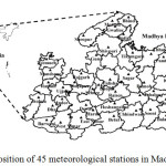
Madhya Pradesh is situated in the center of India covering 443,000 km² of area. Being at the center, the state is surrounded by many other states like Chhattisgarh, Uttar Pradesh, Rajasthan, Gujarat, and Maharashtra. The state is dissected by a major river system, the Narmada which is the lifeline of the state together with Tapti, Mahanadi, Wainganga etc. The area of the state stretches from 21°17' N to 26°36' N latitude and from 74°02' E to 82°26' E longitude. There are 45 districts in the state and the major crops of the region include rice, wheat, jawar, soybean etc. MP has a sub-tropical type of climate with hot dry summer and cool dry winter thus it experiences the extreme climatic condition. Temperature rises to as high as 40°C or more particularly in the southern part in the districts of Khandwa, Khargone etc. In Bhopal, the minimum temperature remains around 25ºC and maximum around 40°C through summer. During winter, the minimum and maximum temperature vary from 10°C to 25°C respectively. The position of the 45 meteorological stations in the state of Madhya Pradesh has been shown in Fig.1.
 

Figure 1: The position of 45 meteorological stations in Madhya Pradesh.  Click here to View figure

Methodology

Analysis of climatic changes over Madhya Pradesh was based on the evalu­ation of available meteorological and hydrological time series using the statistical method (Mann-Kendall method). In the present study testing of the hypothesis, the result shows that the observed historical climatic trends in the central part of India reflected a significant change in climate.

Serial correlation effect

The existence of negative or positive autocorrelation affects the trend in a series (Hamed and Rao, 1998). The autocorrelation (also known as serial correlation coefficients) test was performed to check the randomness and periodicity if any in the time series of all data (Madarres and Silva, 2007). If randomness is found, or in other words, if lag-1 serial correlation coefficients are statistically insignificant then, Mann-Kendall (MK) test is used without altering the authentic data. Otherwise, Modified Mann-Kendall (MMK) test is applied after eliminating the effect of serial correlation (randomness) from the time series (Karpouzos et al., 2010). The autocorrelation coefficient r_k of a discrete time series for lag-k is estimated as follows:

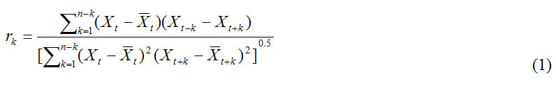
Where, r_k is the lag-k serial correlation coefficient of the series. The hypothesis of serial independence is then tested by the lag-1 autocorrelation coefficient as H₀ : r₁ = 0 against H₁ :|r₁|> 0 using the test of significance of serial correlation (Yevjevich, 1971) following Rai et al., (2010),

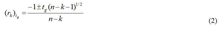
Where,(rk)tg is the normally distributed value of r_k, t_g is the normally distributed statistic at g level of significance. The value of t_g is 1.645, 1.965 and 2.326 at a significance level of 0.10, 0.05 and 0.01 respectively. If |r_k| ≥ (rk)tg the null hypothesis about serial independence is rejected at the significance level α (here 0.05). For the non-normal series, MK test is an appropriate choice for the trend analysis (Yue and Pilon, 2004, Basistha, et al., 2008). Therefore, the MK test has been used wherever the autocorrelation is not significant at 5% significance level.

Pre-whitening

The method of Pre-whiting is applied to remove the effect of Serial correlation on the non-parametric test. Lettenmaier et al., (1994) suggested that the effects of serial correlation upon trend tests in such applications could be assumed negligible; concern about the potential impacts of autoregressive processes upon trend analysis nevertheless appears to be gaining momentum.

Where ^PWX is the whitened data to be used in the subsequent trend analysis and c is the lag-1 serial correlation coefficient as determined directly from the data using Equation 3. Pre-whitening is utilized only if observed r is greater than some critical value, C_criti taken to be 0.1 by von Storch (1995). This method is known as single-stage pre-whitening.

Analysis of trend

The following sections describe the nonparametric (Mann-Kendal) methods used to assess trends over Madhya Pradesh.

Mann-Kendall method

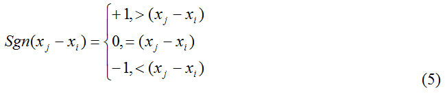
Trend analysis has been executed by using non-parametric Man- Kendall test. It is a statistical method used for analyzing the temporal trends and spatial variation of hydro-climatic series. Smith (2000) mentioned that a non-parametric test is given priority over the parametric one because it can avoid the issue raised by data skew. Man-Kendall test is favored when various stations are tested in the same study (Hirsch et al., 1991). Mann-Kendall test was drafted as a non-parametric test by Mann (1945) for trend detection and test statistic distribution was given by Kendall (1975) for a testing turning point and non-linear trend. The Mann-Kendall statistic S is formulated as

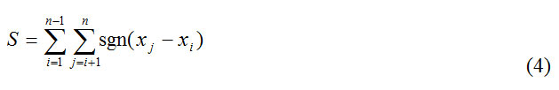
The application of trend test is done to a time series x_i which is ranked from i = 1,2,………n-1 and x_j is ranked from j = i+1,2,……….n. Each of the data point x_i is considered as a reference point which is correlated with all the rest of the data point’s x_j so that
 

The variance statistic is computed as

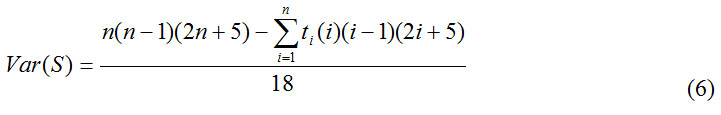
Where t_i represents the number of ties up to sample i. The test statistics Z_c is estimated as

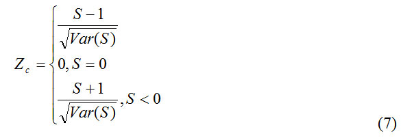
In which Z_c follows a standard normal distribution. A positive (negative) value of Z indicates an upward (downward) trend. A significance level α is also used to test for either an upward or downward monotone trend (a two-tailed test). If Z_c is greater than Z_α/2 where α denotes the significance level, then the trend is significant.

Sen’s Slope Estimator Test

The magnitude of the trend is estimated with the help of Sen’s estimator. In this case, the linear trend is present and hence the true slope is estimated by this method. Here, the slope (T_i) of all data pairs is first computed as (Sen, 1968)
 

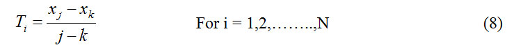
In which x_j and x_k are represented as data values at time j and k (j>k) correspondingly. The median of these N values of T_i is considered as Sen’s estimator of slope which is given as
 

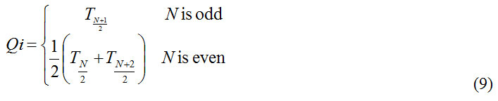
The sen's estimator is calculated as Q_med=T(N+1)/2 if N is odd, and it is computed as Q_med=[T_N/2+T_(N+2)/2]/2 if N is even. Lastly, Q_med is estimated by a two-sided test at 100 (1-α)% confidence interval and then a true slope can be derived by the non-parametric test. Q_i with a positive value indicates an upward or increasing trend and a negative value of Q_i signifies a downward or decreasing trend in the time series.

Mann-Whitney-Pettitt method (MWP)

The time series {X1, X2…, Xn} with length n is taken. t was taken as the time of the most expected change point. Two samples {X1, X2, …, Xt} and {Xt+1, Xt+2, …, Xn} then can be obtained by dividing the time series at t time. The Ut index was obtained in the following way:

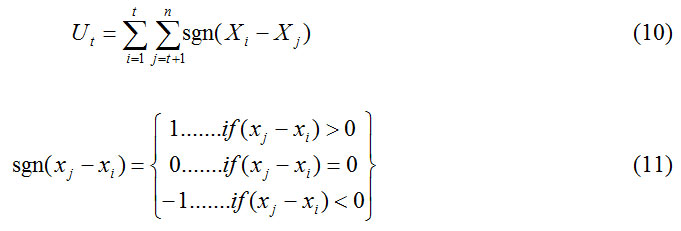
Plotting of Ut value against t in a time series will results in a continuously increasing value of |Ut| with no change point. Yet, if there is a change point (even a local change point), then |Ut| will increase up to the change point level and then will begin to decrease. The major significant change point t gives the point where the value of |Ut | remains highest:
 

The approximated significant probability p(t) for a change point (Pettitt, 1979) is represented as:



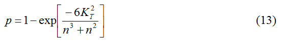
When probability p(t) surpasses (1 – α), then the change point becomes significant statistically at time t with the significance level of α.

Results And Discussion

Lag-1 Serial correlation coefficients of the Annual and seasonal Average Temperature series for entire Madhya Pradesh are represented in Table 1. The annual temperature series almost for all station had a positive lag-1 serial correlation coefficient. As revealed earlier, the existence of positive serial correlation will increase the risk of rejecting the null hypothesis of no trend in the MK test.

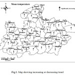
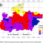
Temperature trend in the region for the period 1901 to 2005 (105 years) showed a significant increasing trend in mean temperature at 5% significance level. During peak summer months the maximum temperature touches 40°C in the entire Madhya Pradesh. Amongst 45 most of the station showed significant increasing trends in mean temperature time series. The magnitudes of annual increase in temperature in the majority of the stations are about 0.001°C. The magnitude of change i.e. Sen’s slope (mm/ year) and percentage change in the trend are presented in Table 2, whereas the positive or negative trend is indicated by the arrow in Fig 2. Results of MK test on the annual average temperature series for all stations are presented in Table 3. The results showed that the monotonic trends in average temperature time series were positive for all stations of Madhya Pradesh. The spatial percentage change in the trends of mean temperature is given in Fig.3. However, the change percentage in trends (increasing) in the case of mean temperature is uniform in larger parts of the state. Homogeneity test has been performed to find the shifting year when a considerable change in the climate was witnessed in the region. Pettitt test is widely used to detect the change year for different series of mean temperature. Table 4 presents series-wise change year for different stations, the tests indicate shifting in the mean categories of temperature were the frequency of occurring years more among 45 stations is the year of 1963. Thus, change point year is 1963 for mean temperature time series for entire Madhya Pradesh, India.

Table 1: Lag-1 serial correlation coefficients of the Annual and seasonal Temperature series for entire Madhya Pradesh (1901-2005)

Table 2: Values of slope β (°C/year) for the Annual and seasonal mean temperature series (1901–2005)

Table 3: Shows Z value obtained by Mann- Kendall Test (1901-2005)

*Bold value indicate significant trend at the 95% of confidence level.

Table 4: Pettitt's  test

Figure 2: Map showing increasing or decreasing trend  Click here to View figure

Figure 3: Map showing percentage change in trend of mean temperature  Click here to View figure

Conclusions

The annual mean temperature time series almost for all 45 station had a positive lag-1 serial correlation coefficient. On another hand, seasonal basis the post-monsoon and winter season also shows the positive correlations were in the premonsoon season most of the station showing a negative trend but in monsoon season only the station betul shows negative correlations among all the station.

Result of MK test confirm that most of the monotonic trends in the annual mean temperature time series were positively significant for all stations at 95% confidence level for entire Madhya Pradesh.

For post-monsoon, pre-monsoon, winter season mean temperature time series increasing significant monotonic trend were found for all 45 stations aspect Monsoon season.

The magnitudes of the significant increasing warming trends in the annual average temperature series were found in the majority of the stations are about 0.01^oC respectively.

Acknowledgment

The authors, thankfully, acknowledges the India Water Portal (Indian Meteorological Agencies) for providing rainfall station data and Department of Science and Technology (DST), New Delhi for providing financial funding during the study period. Due to which quality analysis of average temperature series has been made achievable.

References
 

1. Basistha, A., Arya, D. S. and Goel, N. K., (2008) “Spatial pattern of trends in Indian sub-divisional rainfall”, J. Climatol. , DOI: 10.1002/joc.1706.
   CrossRef
2. Batima, P., Natsagdorj, L., Gombluudev, P. and Erdenetsetseg, B., (2005) Observed climate change in Mongolia. AIACC Working Paper 13, 25.
3. Bhutiyani M.R., Kale, V.S. and Pawar, N.J., (2007) Long-term trends in maximum, minimum and mean annual air temperatures across the north western Himalaya during the twentieth century. Clim Change 85:159–177.
   CrossRef
4. Duhan, D., & Pandey, A., (2013) Statistical analysis of long-term spatial and temporal trends of rainfall during 1901–2002 at Madhya Pradesh, India. Atmospheric Research, 122, 136-149.
   CrossRef
5. Hamed, K.H., and Rao, A.R., (1998) A modified Mann-Kendall trend test for auto correlated Journal of Hydrology 204: 182–196.
   CrossRef
6. Hirsch, R.M., Alexander, R.B. and Smith, R.A., (1991). Selection of methods for the detection and estimation of trends in water quality. Water Resources Research 27, 803-813.
   CrossRef
7. Indrani, P. & Abir, Al-Tabbaa., (2009) Long-term changes and variability of monthly extreme temperatures in India, Accepted: 29 June 2009 / Published online: 12 July 2009 Springer-Verlag 2009.
8. IPCC, (2007) on a scientific basis the contribution of Working Group-I to the Fourth Assessment Report of Inter-governmental Panel on Climate Change (IPCC). Cambridge University Press, Cambridge.
9. Ichikawa, A. (Ed.), (2004) Global warming – The Research Challenges: A Report of Japan’s Global Warming Initiative. Springer, Berlin, 160 p.
   CrossRef
10. Jhajharia, D., Shrivastava, S.K., Sarkar, D., Sarkar, S., (2009) Temporal characteristics of pan evaporation trends under the humid conditions of northeast India. Agricultural Forest Meteorology 149: 763–770.
    CrossRef
11. Jhajharia, D. and Singh, V.P., (2011) Trends in temperature, diurnal temperature range and sunshine duration in Northeast India. Int. J. Climatol. 31: 1353–1367.
    CrossRef
12. Karpouzos, D.K., Kavalieratou, S. and Babajimopoulos, C., (2010) Trend analysis of precipitation data in Pieria region (Greece), European Water, 30: 31-40.
13. Kendall, M.G., (1975) Rank Correlation Methods, 4^th edition. Charles Griffin, London, U.K.
14. Lettenmaier, D.P., Wood, E.F. and Wal1is, J.R., (1994) "Hydro-Climatological tends in the Continental United States, 1948-88." Journal of Climate,7:586-607.
    CrossRef
15. Luterbacher, J., Dietrich, D., Xoplaki, E., Grosjean, M. and Wanner, H., (2004) European seasonal and annual temperature variability. Trends Extremes Sci. 303 (5663), 1499–1503.
16. Mann, H.B., (1945) Non-parametric test against the trend. Econometrica 13, 245–259.
    CrossRef
17. Mishra, N., Khare, D., Shukla, R., and Singh, L.,(2013) “A Study of Temperature Variation in Upper Ganga Canal Command”, published in International Journal of Advances in Water Resource and Protection (AWRP) Volume 1 Issue 3, PP.45-51.
18. Modarres, R. and da Silva, R.V.P. (2007) Rainfall trends in arid and semi-arid regions of Iran. Journal of Arid Environment 70, 344–355.
    CrossRef
19. Pettitt, A.N., (1979) A non-parametric approach to the change-point detection. Appl. Statist. 28(2), 126-135.
    CrossRef
20. Peterson, B.J., Holmes, R.M., McClelland, J.W., Vorosmarty, C.J., Lammers, R., Shiklomanov, A.I., Shiklomanov, I.A. and Rahmstorf, S., (2002) Increasing river discharge to the Arctic Ocean. Science 298, 137–143.
    CrossRef
21. Rai, R. K., Upadhyay, A., and Ojha, S. P., (2010) Temporal Variability of Climatic Parameters of Yamuna River Basin: Spatial Analysis of Persistence, Trend, and Periodicity, The Open Hydrology Journal, 4, 184-210.
    CrossRef
22. Reiter, A., Weidinger, R., Mauser, W., (2012) Recent Climate Change at the Upper Danube - A temporal and spatial analysis of temperature and precipitation time series. Climatic Change 111:665–696.
    CrossRef
23. Revadekar, J.V., Kothawale, D.R., Patwardhan, S.K., Pant, G.B. and Rupakumar, K., (2011) about the observed and future changes in temperature extremes over India. Nat Hazards 66(3):1133–1155. doi:10.1007/s11069-011-9895-4.CrossRef
24. Savelieva, I.P., Semiletov, L.N., Vasilevskaya, Pugach, S.P., (2000) A climate shift in seasonal values of meteorological and hydrological parameters for northeastern Asia. Prog. Oceanogr. 47, 279–297.
    CrossRef
25. Sen, P.K., (1968) Estimates of the regression coefficient based on Kendall’s tau. Journal of American Statistical Association 39, 1379–1389.
    CrossRef
26. Shi, Y.F., Shen, Y.P. and Hu, R.J., (2002) Preliminary study on the signal, impact, and foreground of the climatic shift from warm-dry to warm-humid in Northwest China. J. Glaciol. Geocryol. 24, 219–226.
27. Shukla, R., Deo, R., & Khare, D., (2015, December). Statistical downscaling of climate change scenarios of rainfall and temperature over Indira Sagar Canal Command area in Madhya Pradesh, India. In Proceedings of the 2015 IEEE 14^th International Conference on Machine Learning and Applications (pp. 313-317). IEEE Computer Society.
28. Shukla, R. & Khare, D., (2013) "Historical trend investigation of temperature variation in Indira Sagar canal command area in Madhya Pradesh (1901–2005)" International Journals of Advanced Information Science and Technology (IJAIST), ISSN: 2319:268, Vol.15, No.15.
29. Smith, L.C., (2000) Trends in Russian Arctic river-ice formation and breakup, 1917 to 1994. Physical Geography 20 (1), 46–56.
30. Vincent, L.A., Wijngaarden, W.A.V. and Hopkinson, R., (2007) Surface temperature and humidity trends in Canada for 1953–2005. J. Climate 20, 5100–5113.
    CrossRef
31. Von Storch, H., and Navarra, A., (1995) Analysis of Climate Variability—Applications of Statistical Techniques. Springer-Verlag: New York.
    CrossRef
32. Yevjevich, V., (1971) Stochastic Processes in Hydrology. Water Resources Publications, Fort Collins: CO.
33. Yue, S. and Pilon P., (2004) A comparison of the power of the t-test, Mann-Kendall and bootstrap tests for trend detection. Hydrological Sciences Journal 49(1): 21–37.
    CrossRef