Climate Simulation Using RCM Data for Jamnagar District
Hina Bhatu1 * and Harji Rank2
1
Department of Agriculture,
School of Engineering,
RK University,
Rajkot,
India
2
AICRP on Irrigation Water Management,
Junagadh Agricultural University,
Junagadh,
India
http://dx.doi.org/10.12944/CWE.12.2.25
Scarcity of water resources and pollution will be the major emerging issues in the current and next century. Climate change is also one of the threats among several other impacting on water resources. GCMs are fundamental tools for predicting future climate and RCMs are outstanding tools for studying the mechanisms of climate at scales that are not yet resolved by GCM. The meteorological data (precipitation and temperature) simulated by CGCM2.3.2 RCM for the control period (1961-2000) as well as future periods (2046-64 & 1981-2100) were analyzed for the bias corrections. It was analyzed to assess how well the important statistics (Coefficient of Variation and Mean) of the bias corrected for four grid points of RCM simulated data match those of the observations. The bias corrected RCM simulated rainfall and temperature were found increasing from 1961 to 2100 and noticed that the warming will be more due to increase in minimum temperature rather than maximum temperature.
Copy the following to cite this article:
Bhatu H, Rank H. Climate Simulation Using RCM Data for Jamnagar District. Curr World Environ 2017;12(2). DOI:http://dx.doi.org/10.12944/CWE.12.2.25
Copy the following to cite this URL:
Bhatu H, Rank H. Climate Simulation Using RCM Data for Jamnagar District. Curr World Environ 2017;12(2). Available from: http://www.cwejournal.org/?p=17204
Download article (pdf) Citation Manager Publish History
Introduction
Climate change is also one of the threats among several other impacting on water resources. Scarcity of water resources, pollution and climate change will be the major emerging issues in the current and next century. Climate change and global warming is the result of a build-up of greenhouse gases (GHG), chiefly carbon dioxide, in the atmosphere. Global climate models (GCMs) are fundamental tools for predicting future climate to enable developing a better understanding of climate change.9 Regional climate models (RCMs) are outstanding tools for studying the mechanisms of climate at scales that are not yet resolved by general circulation models (GCM). RCMs are still prone to biases and the simulated climate is not always fully consistent with the observations, which is critical in climate change impact research.14 Several methodologies have been recently proposed and evaluated, mostly focused on precipitation and temperature.1,2,8,13,16
The study area is Jamnagar district of Saurashtra region of Gujarat. It extends from 21º40' N to 22º57' N latitude and 68 º 57' E to 70 º 37' E longitudes. The historical hydro-metrological data (1961-2000) were collected from the State Water data Centre, Gandhinagar and Millet Research station, JAU, Jamnagar. The future weather data simulated by CGCM 2.3.2 RCM for the IPCC SRES-A1B (balance scenario was downloaded from website as detailed by.6,7
Materials and Methods
The bias correction of RCM simulated data was made to match with the observed weather (daily Precipitation and maximum/minimum temperature) for the base line period-1961-2000. Accordingly, the bias correction was applied for the future scenarios-2046-64 and 2081-2100. The mean and coefficient of variation (CV) for the bias correction was applied to the daily minimum/maximum temperature and precipitation on monthly window using the auto correlation by Linear Transformation and & Variance Scaling for temperature and power Transformation for precipitation.
The RCM simulated data were available for 1961-2000 as control period and 2046-64 and 2081-2100 as future predictions. Therefore, for the bias corrections, the period 1967-2000 and 1976-2000 were taken as baseline periods for the temperature and precipitation respectively. The RCM simulated and observed data were compared on monthly window and the statistical parameters namely mean and standard deviations were determined for each of 12 months separately such that both could be matched on monthly windows. The RCM simulated data of the rest periods were bias corrected using the parameters obtained during base line period. The methodology described by17 was used for the bias correction.
Linear Scaling Approach for Precipitation and Temperature
This approach worked for Monthly correction based on the differences between observed and present-day simulated values.12
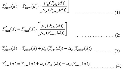
Where,
P*contr(d) = Final bias corrected daily precipitation for RCM simulated 1976-2000.
P*scen(d) = Final bias corrected daily precipitation for RCM simulated 2046-64 and 2081-2100
Pcontr(d) = Daily precipitation for RCM simulated 1976-2000.
Pscen (d) = Daily precipitation for RCM simulated 2046-2064 and 2081-2100
T*contr(d) = Final bias corrected daily Temperature for RCM simulated 1967-2000
T*scen(d) = Final bias corrected daily Temperature for RCM simulated 2046-2064 and 2081-2100.
μm = mean within monthly interval.
Pobs(d) = Daily precipitation for Observed data 1976-2000.
Tobs(d) = Daily Temperature for Observed data 1967-2000.
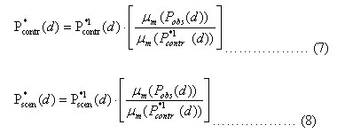
Power Transformation of Precipitation
The variance statistics of a precipitation time series adjust by apb.10,11 First, b was acknowledged by corresponding the CV of the corrected daily RCM precipitation (Pb) with the CV of observed daily precipitation (Pobs) for each month m. The value of bm was taken as
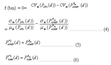
According to Brent’s method3 it is done by root-finding algorithm. By using the standard linear scaling parameter the long-term monthly mean of observed precipitation was matched with the monthly mean of the intermediary series P*1contr(d)
Variance Scaling of Temperature
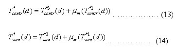
The mean and the variance effectively corrected by Power transformation. Due to the use of a power function, it is limited to precipitation time series. The means (μm) of the RCM-simulated time series were adjusted by linear scaling (Eqs. (3) and (4))4, 5 Meanwhile, the mean-corrected control (T*1contr(d)) and scenario runs (T*scen(d))were shifted on a monthly basis to a zero mean.
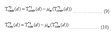
Then, Based on the ratio of observed σ and controlrun σ the standard deviations of the shifted time series (T*2contr(d) and T*2scen(d)) were scaled.
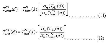
And finally, the σ-corrected time series (T*3contr (d) and T*3scen(d)) were shifted back using the corrected mean (μm (T*1contr(d)) and μm (T*1scen (d))) of step one:
Results and Discussion
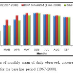
Precipitation for control Scenario (1976-2000)
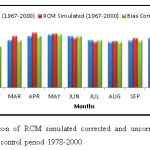
The Fig.1 shows that the RCMs simulated daily precipitations were found overestimated over actual observation during May to July. However, after applying bias correction, the monthly daily mean, standard deviation and coefficient of variation of daily precipitation for each of 12 months was exactly matched with those of respective observed data for the base line period of 1976-2000. The uncorrected RCMs precipitation had a positive (Over Estimated) bias from May and June and biases for the July and August months were negligible. In comparison to the corrected RCMs output, the uncorrected monthly mean precipitation values were higher during May and June months and nearly same during July and September month.
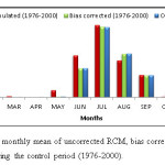 |
Figure 1: Comparison of monthly mean of uncorrected RCM, bias correctedRCM and observed daily precipitation during the control period (1976-2000). Click here to View figure |
The effect of sampling variability was reduced by determining the parameters a and b for every month of the year using the distribution free approach. Determination of the parameter b was done iteratively, so that the coefficient of variation of the daily precipitation values predicted by RCM matches the coefficient of variation (CV) of the observed monthly precipitation. Parameter a was determined such that the mean of the transformed daily values of precipitation matched with the observed mean. A depended on b and b depended only on CV 15. Fig.2 displays the annual cycle of the coefficient a and exponent b for four grid points of RCM run for the control period.
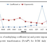 |
Figure 2: The comparison of multiplying coefficient (a) and power exponent(b) for correcting the biases through power transformation (P1=aPb) for RCMdaily precipitation during different months. Click here to View figure |
Precipitation for Future Scenario (2046-2064)
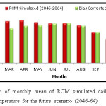
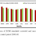
Fig.1 shows the precipitation simulations and bias corrected precipitation varied considerably during the control period 1978–2000. When the analysis was performed using raw data without bias correction, RCMs showed a higher amount of disagreement during April and May months in 2046-64 (Fig.3). By the bias correction of RCM simulated precipitation, the monthly mean of the daily corrected values were reduced over simulated raw values during the April and May months. For the rest of months, the values did not differed much.
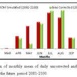
Precipitation for Future Scenario (2081-2100)
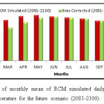
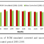
In Fig. 4, the bias corrections of simulated raw data reduced the precipitation amounts than of original amount simulated by RCM during April and May Months. Meanwhile, during August and October Months the corrected precipitation was higher than that of uncorrected.
When the analysis was performed using raw data without bias correction, RCM simulations showed a large amount of disagreement. Thus, the range of projected future percentage changes in precipitation differed a lot from May to August. On an average, precipitation is expected to increase during July and August as compared to RCMs simulated, whereas it is projected to nearly same for all other seasons. The largest corrections were required in May, for which the mean precipitation was reduced to 1.97 from 8.45.
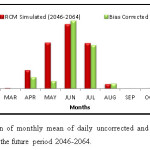 |
Figure 3: The comparison of monthly mean of daily uncorrected and corrected precipitation simulated by RCM for the future period 2046-2064 Click here to View figure |
 |
|
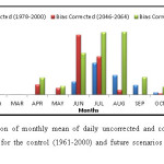
Comparison of precipitation for control (1976-2000) and future scenarios (2046-2064 and 2081-2100)
Fig. 5 showed that the monthly mean of daily precipitation in the months of April to July would be increased during 2046-64 as compared to base line period-1976-2000. During future-2081-2100, the months of April, July, August, September and October were increased as compared to period of 2046-64 and base line period-1976-2000. During 2081-2100, in June Months is reduced over period of 2046-64. However, it will be highest during the period-2081-2100 followed by 1961-2000 and 2046-64 during the months of July to October. Therefore, it can be said that the rainfall during July to October will be reduced during the period 2046-64 as compared to base line period-1961-200 and again it will be increased during the period-2081-2100. There can be no much impacts on rainfall during the Months of January to March, November and December.
 |
|
Minimum Temperature for Control Scenario (1967-2000)
Figure 6 shows that the RCMs simulated minimum temperature were overestimated during January to May and December months. After applying the bias correction of Linear Transformation and Variance Scaling methods, the mean and CV of the daily minimum temperature were agreed well with the actual observations for whole year. It was found that the RCM in simulating the daily minimum temperature had a positive bias from January to May and December months.
Minimum Temperature for Future Scenario (2046-2064)
Fig.7 shows that the RCM simulated daily minimum temperature higher during the months of January to May and December which required to be bias corrected. While during the rest of the months, the uncorrected and corrected daily minimum temperature did not differed much. The RCM simulated daily minimum temperatures during the months of January to May and December were reduced after bias corrections.
Minimum Temperature for Future Scenario (2081-2100)
Fig 8 shows that the RCM simulated the daily minimum temperature are higher during the months of January to May and December which required to be bias corrected. While during the rest of the months, the uncorrected and corrected daily minimum temperature did not differed much. The RCM simulated daily minimum temperatures during the months of January to May were reduced after bias corrections. The bias corrected daily minimum temperature was decreased over the uncorrected.
 |
|
 |
|
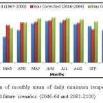
Comparison of Minimum Temperature during baseline period (1967-2000) and future scenarios (2046-2064 and 2081-2100)
Fig. 9(a) shows that the daily minimum temperature would be increased day by day due to global warming during the most of the April to August months of the year. During January to March and September to December months, the temperature will increase during the 2046-64 and again it will decrease during 2081-2100 over 2046-64. However, the highest warming due to minimum temperature will be in 2046-64 for the months of January to March & December followed by 2081-2100 and 1961-2000. During the month of September to November, the minimum temperature will be highest during 2081-2100 followed by 1961-2000 and 2046-64.
 |
|
 |
|
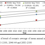
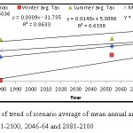
The average of mean annual and seasonal mean-Tmin during the overall scenarios (1961-2100) presented in Fig. 9(b) and it showed that the mean Tmin during annual, winter, summer and monsoon season was found as increasing at 3.6 0C per century, 4.4 0C per century, 4.1 0C per century and 2.2 0C per century (The scenario average values are taken at middle of scenario).
Maximum Temperature for Control Scenario (1967-2000)
Fig.10 shows that the RCM simulated uncorrected daily maximum temperature was higher during the months of January to May, august and September and lower during June to October and November than the actual observed data.
 |
|
 |
|
Maximum Temperature for Future Scenario (2046-2064)
Fig. 11 shows that the RCM simulated the higher maximum temperature during February to May, August, September and December while lower during June, July, and November. During the rest of the months, the uncorrected maximum temperature did not differ much from corrected data.
Maximum Temperature for Future Scenario (2081-2100)
The Fig. 12 shows that the RCM simulated the maximum temperature higher during January-April and September while lower during June, July and November and rest the months did not differed much. In fact, the biases in simulating the maximum temperature during the entire year could not found much.
 |
|
 |
|
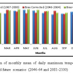
Comparison of maximum Temperature during baseline period (1967-2000) and future scenarios (2046-2064 and 2081-2100)
Fig. 13(a) shows that during the January to March, August and December month, the maximum temperature will be higher during future scenario-2046-2064 over control period-1961-2000 and 2081-2100. However, the maximum temperature will be lower during 2081-2100 over 2046-64 but higher than 1961-2000. During the future 2046-2064, the maximum temperature during April-June and in October months is lower than the control scenario 1961-2000 and future scenario 2081-2100. The highest increase in the maximum temperature in the future can be during the December to March. This can affects the cereal crops sown during the winter season.
 |
|
The average of mean annual and seasonal mean-Tmax during the overall scenarios (1961-2100) presented in Fig. 13(b) and it showed that the mean Tmax during annual, winter, summer and monsoon season was found as increasing at 1.9 0C per century, 3.0 0C per century, 1.4 0C per century and 1.2 0C per century.
 |
|
Conclusions
The increasing rainfall and warming trends were noticed in the study area for the IPCC A1B scenario. The monsoon seasonal rainfall during the period 1961-2000, 2046-64 and 2081-2100 was found as 548mm with an average increasing trend of rainfall at 9.3mm/year from 1961 to 2100.The annual, winter, summer and monsoon seasonal average of daily minimum temperature were found increasing at 3.6 0C per century, 4.4 0C per century, 4.1 0C per century and 2.2 0C per century. The annual, winter, summer and monsoon seasonal average of daily maximum temperature during annual, winter, summer and monsoon season was found as increasing at 1.9 0C per century, 3.0 0C per century, 1.4 0C per century and 1.2 0C per century. The warming trend was found more due to daily minimum temperature rather than maximum temperature.
Acknowledgement
I hereby express my heartfelt gratitude my advisor Dr. H. D. Rank and my sincere thanks to Bhaskaracharya Institute for Space Application and Geo- Informatics (BISAG), Gandhinagar, State Water Data Centre (SWDC), Gandhinagar and Millet Research station, JAU, Jamnagar for extending help in data procurements.
References
- Berg P, Feldmann H and Panitz, H J. Bias correction of high resolution RCM data. Hydrol. 448–449: 80–92(2012).
CrossRef - Bordoy R. and Burlando Bias Correction of Regional Climate Model Simulations in a Region of Complex Orography. J. Appl. Meteorol. Clim.52:82–101(2013).
CrossRef - Brent, R.P. An algorithm with guaranteed convergence for finding a zero of a function. J. 14 (4): 422–425 (1971.)
- Chen J, Brissette F P and Leconte R. Uncertainty of downscaling method in quantifying the impact of climate change on hydrology. Hydrol. 401 (3–4):190–202 (2011a).
CrossRef - Chen J, Brissette F P, Poulin A and Leconte R. Overall uncertainty study of the hydrological impacts of climate change for a Canadian watershed. Water Resour. Res.47 (12) (2011b).
CrossRef - Dile Y T and Srinivasan R. Evaluation of CFSR climate data for hydrologic prediction in data-scarce watersheds: an application in the Blue Nile River Basin. Journal of the American Water Resources Association (JAWRA)1-16 (2014.)
- Fuka DR, MacAllister, C A,Degaetano A T and Easton Z M. Using the Climate Forecast System Reanalysis dataset to improve weather input data for watershed models. Proc.DOI: 10.1002/hyp.10073 (2013).
CrossRef - Haerter J O, Hagemann S, Moseley C and Piani C. Climate model bias correction and the role of timescales. Earth Syst. Sc., 15: 1065–1079, doi: 10.5194/hess-15-1065- 2011 (2011).
- Kundzewicz Z W, Mata L J, Arnell N, Doll P, and Jimenez B. The implications of projected climate change for freshwater resources and their management. HydrolSci J. 53: 3-10 (2008).
CrossRef - Leander R and Buishand T A. Resampling of regional climate model output for the simulation of extreme river flows. Hydrol. 332 (3–4): 487–496 (2007).
CrossRef - Leander R, Buishand T A, van den Hurk, B JJ M and de Wit M JM. Estimated changes in flood quantiles of the river Meuse from resampling of regional climate model output. Hydrol.351 (3–4): 331–343 (2008).
CrossRef - Lenderink, G.; Buishand, A. and Van Deursen, W. Estimates of future discharges of the river Rhine using two scenario methodologies: direct versus delta approach. Earth Syst. Sci.11 (3): 1145–1159 (2007).
CrossRef - Piani, C.,Haerter J and Coppola E.Statistical bias correction for daily precipitation in regional climate models over Europe. Appl. Climatol.99: 187–192 (2010a).
CrossRef - Portoghese I, Bruno E, Guyennon N and Iacobellis Stochastic bias-correction of daily rainfall scenarios for hydrological applications. Nat. Hazards Earth Syst. Sci.11: 2497– 2509.doi:10.5194/nhess-11-2497-2011 (2011).
CrossRef - Raneesh K Y and Thampi S G. Bias Correction for RCM Predictions of Precipitation and Temperature in the Chaliyar River Basin. J Climatol Weather Forecasting. 1(2) (2013).
- Terink W, Hurkmans R T W L,Torfs P J J F and Uijlenhoet R. Evaluation of a bias correction method applied to downscaled precipitation and temperature reanalysis data for the Rhine basin. Earth Syst. Sci. 14: 687–703.doi:10.5194/hess-14-687- 2010 (2010).
- Teutschbein C and Seibert J. Bias correction of regional climate model simulations for hydrological climate-change impact studies: Review and evaluation of different methods. Journal of Hydrology 456–457: 12–29 (2012).
CrossRef


