Land-Use and Land Cover Changes on the Slopes of Mount Meru-Tanzania
Aldo Japhet Kitalika 1
*
 , Revocatus Lazaro Machunda 1
, Hans Charles Komakech 1
and Karoli NIcholas Njau 1
, Revocatus Lazaro Machunda 1
, Hans Charles Komakech 1
and Karoli NIcholas Njau 1
1
Department of Water and Environmental Science and Engineering,
Nelson Mandela African Institution of Science and Technology,
Tengeru- Arusha,
P.O.BOX 447
Tanzania
http://dx.doi.org/10.12944/CWE.13.3.07
The study of spatial land use and land change is inevitable for sustainable development of land use plans. Environmental transitions analysis was done in part of the land on the slopes of the foothills of Mount Meru in thirty (30) years’ time from 1986 to 2016 using satellite-derived land use/cover maps and a Cellular Automata (CA) spatial filter under IDRISI software environment and assessed the important land use changes. Also, the future land use for 2026 which is the next ten (10) years was simulated based on Cellular-Automata Markov model. The results showed significant land use transitions whereby there is a huge land use change of bush land (BL) and agriculture land (AG) into human settlement (ST) which resulted into conversion of Arusha town into a City. In addition, the changes have caused slight changes in water bodies into mixed forest. Moreover, the future land use/land cover (LULC) simulations indicated that there will be unsustainable LULC changes in the next ten years since most of bush land and part of agriculture land will be used for building different structures thus interfering with fresh water and food availability in the City. These changes call upon the relevant planning authorities to put in place the best strategies for good urban development.
Copy the following to cite this article:
Kitalika A. J, Machunda R. L, Komakech H. C, Njau K. N. Land-Use and Land Cover Changes on the Slopes of Mount Meru-Tanzania. India. Curr World Environ 2018;13(3). DOI:http://dx.doi.org/10.12944/CWE.13.3.07
Copy the following to cite this URL:
Kitalika A. J, Machunda R. L, Komakech H. C, Njau K. N. Land-Use and Land Cover Changes on the Slopes of Mount Meru-Tanzania. India. Curr World Environ 2018;13(3). Available from: https://bit.ly/2DBOu9o
Download article (pdf)
Citation Manager
Publish History

In the modern world, LULC is inevitable since human use their environment for their development. Human may use the atmosphere, surface and underground of the earth for development and on doing so they may affect the environment. Such changes occur as a result of complex processes that involve modifications in land-cover and land use,1 and they are determined by the interaction in space and time between biophysical and humans endeavors.2 Such processes include but not limited to expansion of agriculture, infrastructures, settlements, development of industries and natural disasters. In several areas on the earth, river ecosystems and land cover have changed as a result of various forces persisting on them which have led to modification of the flow regime,3,4 and change in ecology. Such forces include deforestation, overgrazing, expansion of agriculture, and infrastructure development. Moreover, the increased competition for water use and conversion in land use in the upstream of many rivers are said to have contributed to change in hydrological regimes of many rivers and wetlands.5,6 Different government policies, political influences as well as technological changes can also lead to land use/land cover changes which can affect the watersheds and catchment areas.3,7,8 The above-mentioned issues are among of the several activities degrading large environment in many developing countries including Tanzania.
The study on impacts of land-use and land cover change has been a point of interest of many researchers. For example,2,9–11 on their studies attempted to provide the insights and understanding of the causes and effects of land-use and land cover change with most emphasis of their studies on biophysical aspect of land-use and land cover change. Currently, large areas in Nothern Tanzania are said to have been converted to agricultural land and other uses, including the cultivation of food and cash crops, overgrazing, expansion of settlements and development of infrastructures such as irrigation scheme systems, mining and other industries as a result of increased migrations and internal population. Such areas include the slopes of Mount Meru in Tanzania which is among the important Pangani basin sub catchment feeding the Pangani River.12,13 This area is facing deforestation and forest degradation, poor agricultural expansion which includes increased furrow irrigation technology, establishment of new large commercial farms from virgin land, overgrazing, rapid increase in human population due to immigration and natural process threatened the land use and land cover of the area hence affecting the hydrological system of the area.6,13,14 Currently, there has been a significant increase of farming and livestock activities in the Pangani basin sub catchment. This has raised the dramatic conversion of grassland, woodland and forest into cropland and pasture which eventually results into negative changes in the wetlands size and river regimes.6
Knowing the main drivers of land use and land cover change on rivers and its aspects is vital, such understanding includes both assessments of the expected rate and spatial pattern of land-use and land-cover change (LULC) as well as familiarity of the principal human and biophysical drivers.2 These complex questions can be answered through modeling the land use land cover change in GIS environment. Also, the process of analysis, forecasting and evaluating future land-use change of any place involves a complicated set of tasks, and should be performed using better scientific knowledge of the physical extent, character and consequences of land transformation.15 In analysis and modeling of LULC dynamics, remote sensing and GIS tools are widely used to study both quantitatively and qualitatively using Cellular Automata and Markov Chain (CA-MC) spatial models and predicting the future LULC scenario basing on historical land cover data.10,16–19 Apart from that, Normalized Difference Vegetation Index (NDVI), principal component analysis (PCA), image rationing, image differencing, change vector analysis in terms of magnitude and direction, deviation and regression, are among the techniques which can be used in GIS environment to study the LULC changes.17,20,21 In this study, CA-MC has been used to assess the land use change and model the future LULC in part of the Pangani basin catchment.
Land Cover Change and Drainage
Land cover plays a vital role in drainage system and conservation of any catchment. Different studies have shown the land covered with different types of vegetations in relation to soil type can affect the drainage and sustainability of a particular catchment.22,23 Further studies by different researchers have shown that the pressure for change in a land cover can particularly cause changes in the hydrological regime of an area especially when extensive deforestation has taken place.24 While this happen, the catchments study shows that the hydrological regime of an area can change with no significant changes of precipitation over long time.25 Other studies show stream annual flow to be high in forested areas than deforested area but does not show the season in which such events occurs.26
Cellular Automata
CA is one of the methods used to model land change in terms of geospatial location of development as well as quantity of change. In this model, the geospatial dynamics are controlled by local rules determined either by the CA spatial filter or transition potential maps.27 The CA model is defined as a one or two-dimensional grid of identical automata cells of which each automata cell processes respective information, and proceeds in its actions based on data received from its environment and following rules that it stores or holds internally.28 A simple CA have five components which are the grid space on which the model operates, cell states in the grid space and transition rules, which determine the spatial dynamic process. Others include status of neighborhoods that influences the central cell and iteration numbers.29 In addition, a grid of automata must be defined by a set of inputs from the states of neighbouring cells to become a CA. Moreover, two-dimensional CA must be considered on a grid lattice with the influencing neighborhoods containing four (von Neumann function) or eight (Moore function) adjacent cells.30 The most important advantage of the CA models is based on its ability to control complex spatially distributed processes, as well as affording insights into a wide variety of local behaviors and global patterns. Furthermore, temporal and spatial complexities of many phenomena can be well simulated and represented by properly defining transition rules in CA models.29 With such vital advantages, CA models have been increasingly used for simulating different spatial phenomena including LUCC31 and urban growth.32 These features give most significant concern in CA modeling which requires defining appropriate transition rules based on training data which control the model. Furthermore, linear boundaries have been used to define the rules; however, land-use dynamics, and many other geospatial phenomena, are extremely complex and require non-linear boundaries for the definition of rules.29
Markov Chain Model
The Markov Chain premise is a stochastic series that depicts the probability of how one state is altered to another state. The Markov Chain produces a key descriptive outcome that determines the probability of change from one category to another category thus managing the temporal dynamics among the land use/cover categories, based on transition probabilities (e.g. conservation to built-up area), which is a also called transition probability matrix.10,33 This model is highly used for studies of water resource systems and simulation of precipitation sequences, particularly to describe and predict lithological transition,34 plant succession35 and land use change.36 The model works under assumption of several mathematical probability theories of transition probabilities calculated through the Chapman-Kolmologov equation. In this study, such mathematical manipulations are omitted since GIS softwares are used for the same purpose.
CA- Markov Chain Model
The CA-MC model is an integrated system which plays a great role in multi-criteria evaluation of LULC changes. It is among the best method and technique for quantity estimation, spatial and temporal dynamic modeling of LULC changes since GIS and remote sensing data can be well integrated to give a meaningful outcome.33 In this model, the MC tool is used to produce transitional probabilities statistics, transitional area statistics and conditional transition images data which are used as inputs to predict the later state of the particular pixels over space basing on the condition, location and proximity of the neighboring pixel in CA model.10,16,18,19,37–40 In this paper, studies on the impacts of land use and land cover changes on water resources on the slopes of mount Meru is assessed using CA-MC spatial models. The two models will be used to estimate and project the future land cover land use changes of the study area.
Materials and Methods
Description of Study Area
The study area involved the foothills of the eastern and south west parts of Mount Meru which is part of the entire Pangani basin sub catchment located in the Nothern part of Tanzania sub catchment (Figure 1).41 The natural vegetation in this area is typically tropical forest to savannah and topography is dominated by the Mount Meru volcanic cone of Pleistocene to recent origin. The local climate of the area is temperate Afro-Alpine with minimum and maximum daily temperature of 20.6 °C and 28.5 °C, respectively. The rainfall is irregularly distributed between a main wet season from February to mid May and a minor one from September to November both giving the mean annual rainfall of 535.3 mm.42,43 The catchment area of the river (headwater) is characterized by both artificial coniferous trees and mixed natural forest conservation; middle area of the river consists of mixed agriculture and urban settlement. The floodplain (downstream) region is characterized by bare land, intensive grazing, large scale agriculture, treated municipal sewage disposal and serious flooding in wet season.44
 |
Figure 1: Location of the study area |
Sources of Data and Data Collection
In this study, both primary and secondary data were used. The primary data used include precipitation and water levels in rivers within the sub catchment for 2016, and the secondary data for precipitation in 1986, 1996 and 2006 were collected from the Pangani Basin Water Office (PBWO) (Table 1). Other secondary data includes the Landsat Thematic Mapper (LTM) images downloaded from United States Geological Survey (USGS) Earth Explorer as shown in Table 2 The collected satellite images were used to determine the change in land use/land cover of the area over time within thirty years (1986-2016). The classified satellite images were also used to predict the condition of land use /land cover condition in 10 years later in the Markov- Cellular Automata dynamic model (MCA).
Data Analysis
The collected satellite images were pre-processed first before analyzing them, the process involved projecting them to UTM zone 36 S which corresponds to Arusha Region, and then the red green and blue (RGB) composite images were created for each year. RGB were created by layer stacking which involved Band 2, 3 and 4 for Landsat TM 4-5 and Band 3, 4 and 5 for Landsat 8. Each image with composite colour was extracted to cover the study area by using the study area map. Images were analyzed by using IDRISI-Selva software and the results were assessed basing on the changes occurred in the land uses and associating them with water reservoirs. The satellite images were preprocessed then converted into composite images with false colors which could help to identify clearly the areas with different land uses like vegetation, settlements and water sources through supervised classification.16,18 Maximum likelihood (MAXLIKE) algorithm was used to classify the images for change detection analysis. Analysis of the net gain and loss of various land uses like forest cover, settlements and agricultural having a time step satellite images were performed and interpreted basing on Kappa Index of Agreement (KIA)10 for the best image representative image of the future land use land change prediction model. The whole procedural activities are summarized in Scheme 1. Also, the rainfall and river water levels for some years were used to evaluate any correlation in relation to land use/land cover change if any.
Satellite Image Classification, Training, Signature Development and Classification
Supervised image classification was adopted due to the fact that the whole process is controlled by the user especially on deciding the number of classes to be identified, creation of training samples and detailed knowledge about the real study area land use and land cover distribution.45 The training samples representing the pixels with particular land covers for 1986, 1996, 2006 and 2016 were created by using polygons with the aid of GPS points with support from Google earth image. In addition, the land use topographic maps for similar years representing the study area for Quarter Degree Square (QDS) 55-3 and 55-4 collected from Cartography Department of the Ministry of Land were also used for the same purpose. Six classes of land LULC were identified which involved Mixed forest (MF), Bush land (BL), Agriculture (AG), Settlements (ST), water bodies (WB) and rocks (RK). Twenty five (25) pixels each were used for training and validation of WB and RK whereas for MF, AG and ST fifty (50) pixels were used for the same purpose. The same training samples were stored and used to create signature file for entire image supervised classification process. Table 3 below describes the land use classes identified in the study area.
Table 1: Annual precipitation and discharge in rivers in 1986 to 2016
|
Year |
Ann. Prec. (mm) |
Discharge (m3/s) |
||||
|
Temi |
Nduruma |
Tengeru |
Maji ya Chai |
Av. Level |
||
|
1986 |
503.3 |
0.67 |
0.75 |
0.66 |
0.30 |
0.60 |
|
1996 |
225.4 |
0.29 |
0.34 |
0.28 |
0.13 |
0.26 |
|
2006 |
229.6 |
0.31 |
0.35 |
0.31 |
0.14 |
0.28 |
|
2016 |
464.3 |
0.61 |
0.75 |
0.38 |
0.19 |
0.48 |
Source: Pangani Basin Water Office (PBWO) 2016, Ann. Prec.- Annual Precipitation, Av. - Average
Table 2: USGS collected Landsat TM characteristics used for LULC
|
Satellite Image |
Resolution |
Path |
Row |
Collection date |
|
Landsat TM 4-5 |
30m × 30m |
168 |
062 |
Sep-1986 |
|
Landsat TM 4-5 |
30m × 30m |
168 |
062 |
Sep-1996 |
|
Landsat TM 4-5 |
30m × 30m |
168 |
062 |
Sep-2006 |
|
Landsat ETM 8 TIR/OLI |
30m × 30m |
168 |
062 |
Oct-2016 |
Table 3: Description of land use classification of the study area
|
Land Use |
Description |
|
Mixed Forest (MF) |
Areas with plantation and natural forest, firewood, charcoal, pole wood and timber |
|
Bush land (BL) |
Areas with shrubs, agro forest, pasture and thickets |
|
Agriculture (AG) |
Areas with land for commercial and peasant agriculture |
|
Settlements (ST) |
All forms and types of buildings |
|
Water bodies (WB) |
All areas covered with water (rivers, snow, lakes floods and wastewater treatment sites) |
|
Rocks (RK) |
All areas with rocks and mining |
Supervised image classification was done after creation of signature file; each composite image was supplied in the Maximum Likelihood Classification Algorithm as input together with the associated signature file. After running the Algorithm, the Land use and Land cover maps with trained Classes were produced and was ready for Classification Accuracy Assessment process. All these processes were performed on each individual image in ArcGIS 10.3 software.
Accuracy Assessment and Change Detection Analysis
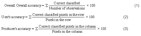
The assessment of classification accuracy was performed on each classified map by comparing the land use classes with 33 ground truth GPS points then creating an error matrix table; the producers, users and overall accuracy were calculated from the table in Microsoft excel sheet, as suggested by Coppin and Bauer (1996), which requires acceptable classification results to be at least from 70% and above. The overall accuracy was determined by the relation given in relation (1) to (3). Table 2.5 gives a summary of accuracy assessment for year 1986 to 2016 which all qualified for further adoption.
Change Detection Analysis
The statistics from classified land use and land cover maps of 1986, 1996, 2006 and 2016 were used to detect the changes occurred in the period of 30 years. Change detection involved finding the quantities of the land use land cover changed, locations where the changes occurred and the type of changes occurred at a certain defined time interval.10,46 In post classification process; quantitative changes were detected by comparing the successive pairs of classified maps by subtracting the quantities of the current land use class from the quantities of the past land use class; the differences obtained from each pair were converted to percentage of change by using relation.4

Through change detection the deep understanding in terms of anthropogenic interference in the land use and land covers of an area will be possible hence this can facilitate in understanding the protection strategy of the environment.
Analysis of LULC
Figures 2 (a) and (b) through 3 (c) and (d) are LULC maps of the study area for 1986, 1996, 2006 and 2016 and their statistics are summarized in Tables 4 through 8. The study shows that agriculture land increased from 46.85% in 1986 of the total land use to 50.42% in 1996 with land use of 545.8 km2 to 587.4 km2, respectively. While this happened, bush land decreased from 31.5% to 24.19% meaning that rise in agriculture occurred in a sacrifice of conversion of bush land. Also within similar years mixed forest increased from 139.7 km2 to 174.9 km2 meaning that maybe part of the bush land was a result of forest clearance which was recovered in the 1996 (Table 4 and 8). In addition, areas inhabited by human settlement increased in the ten years from 74.3 km2 in 1986 to 110.4 km2 in 1996 that being the result of conversion of bush land and part of agriculture area (Table 8). The areas inhabited by water bodies decreased to 0.45% in 1996 from 1.2% for the year 1986. Several reasons may explain as why this happened due to the fact that water bodies are contributed in environment as a result rainfall, precipitations, soil type and the extent of canopy cover which accounts for evaporation index. Rainfall being the main source of surface water, then it is anticipated that fluctuation of rainfall could be the best reason explaining the extent and existence of water bodies on surfaces.
The agriculture land decreased in 2006 with only 42.8% being used up compared to 50.42% in 1996. The cross-tabulation study shows that the agriculture land was partly converted to bush land (15.5 km2 uncultivated for long time and changed to bush land) and 90.6 km2 was converted to settlement as a result of urbanization. Generally, settlements increased by 96.8 km2 and 53.9 km2 in 2006 and 2016, respectively (Table 7 and 8). However, in ten years later (2016) agriculture was stimulated to 45.62 % (increase by 2.82% with a net gain of 32.8 km2) due to decreased rates of settlements constructions and part of the bush land was reconverted into agriculture land (Figure 3(d) and 10, Table 4 and 8). More analysis shows mixed forest (MF) conservation decreased consecutively between 1996 and 2016 but in a decreasing rate by 8.2 km2 for the year 1996 to 2006 and 0.7 km2 in ten years later. That means that between 2006 and 2016 forest conservation was strongly put in place to rehabilitate parts of the bush land into forest or to increase the plantation forest in bush lands. Such improved forest plantations include the Midawe and Temi waterfalls catchment areas where big estates of coniferous (pines) trees were raised. Also, the water bodies (WB) continued to decrease up to 10.6 km2 by 2006 whereas in 2016 it increased by 0.8 km2. That being a ten years case, generally the water bodies have decreased in 30 years (1986-2016) by 9.8 km2 which can be a global alarming situation. It should be noted that most rivers running in Arusha City have their main catchment sources being within the top hills of mount Meru which is part of the study area and therefore it is an area of profound importance in terms of fresh water sources. A close examination of LULC maps of the study area from Figures 2 and 3 show a progressive decrease of water bodies at the top hills which can be associated with melting of the ice caps, decreased precipitation, increased atmospheric temperature and evaporation. It is very unfortunate that different scholars had different ideas on the effect of canopy cover towards the water bodies whereby some scholars advocates increase in rivers discharge with increased deforestations25 and others arguing differently.26 While these arguments remain contradictory, it should be remembered that runoff always increase with deforestation due to decrease of water breaks hence infiltrations. Also, soil conditions (sandy, clay, loamy or rocks) account for water infiltration as a main source of rivers and aquifer recharge (Soil and Water Analysis Tool, SWAT). Loose soil is likely to allow more infiltration than compact soil and the vice versa is true. The proportions of change of each LULC category for the year 1986 to 2016 are summarized in Table 7.
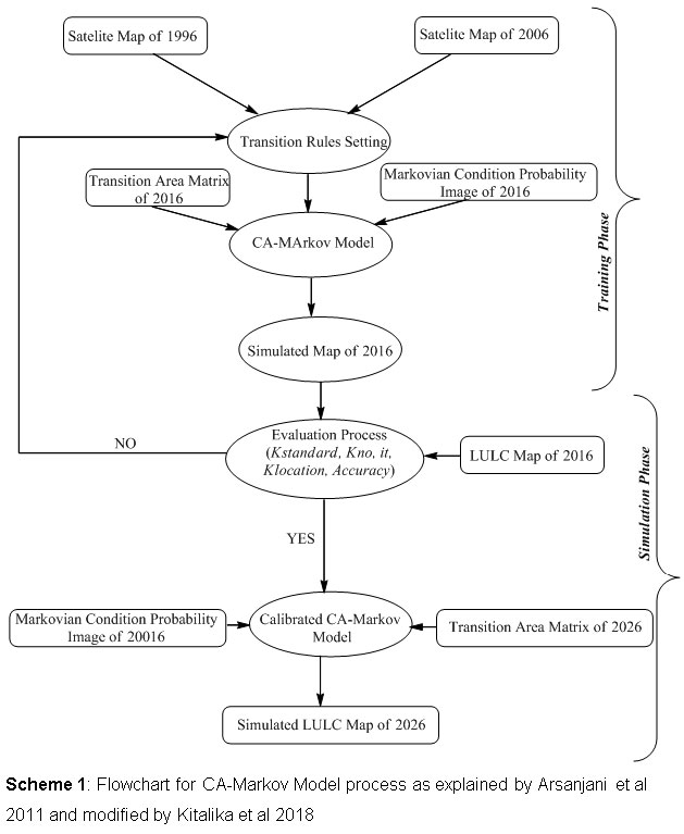 |
Scheme 1: Flowchart for CA-Markov Model process as explained by Arsanjani et., al 2011 and modified by Kitalika et., al 2018 Click here to view Scheme |
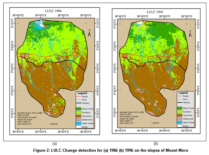 |
Figure 2: LULC Change detection for (a) 1986 (b) 1996 on the slopes of Mount Meru Click here to view figure |
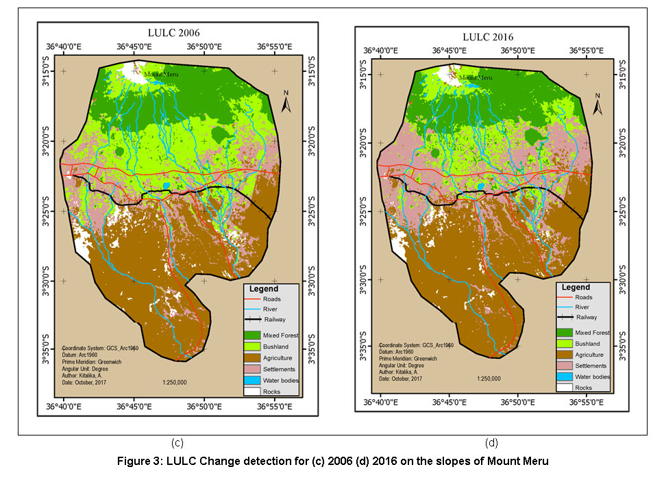 |
Figure 3: LULC Change detection for (c) 2006 (d) 2016 on the slopes of Mount Meru Click here to view figure |
 |
Figure 4: Cross tabulation for LULC change detection on the slopes of Mount Meru from 1986 to 1996 Click here to view figure |
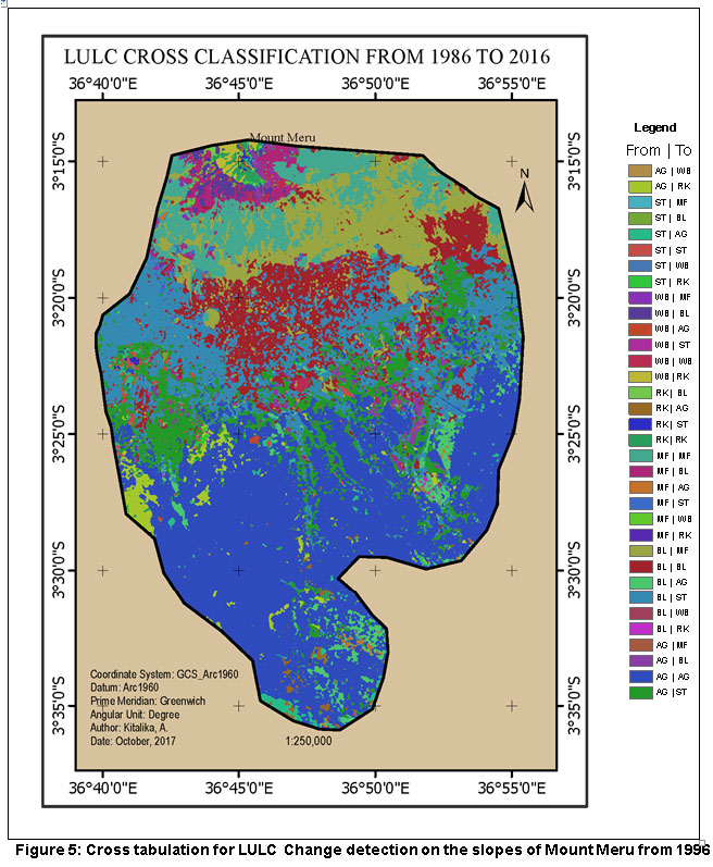 |
Figure 5: Cross tabulation for LULC Change detection on the slopes of Mount Meru from 1996 to 2006 |
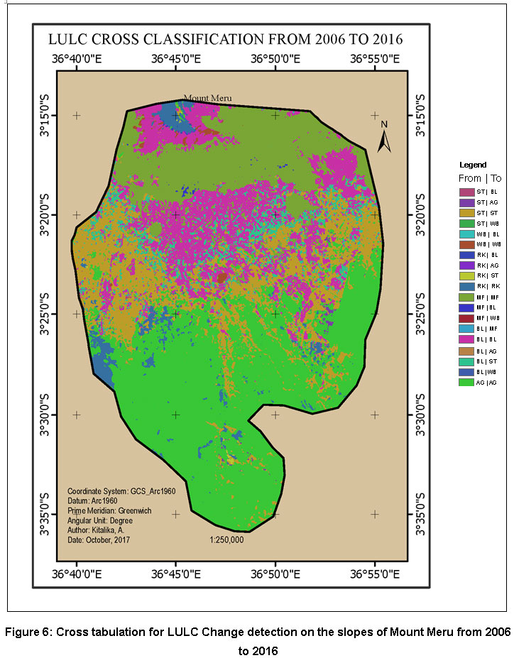 |
Figure 6: Cross tabulation for LULC Change detection on the slopes of Mount Meru from 2006 to 2016 |
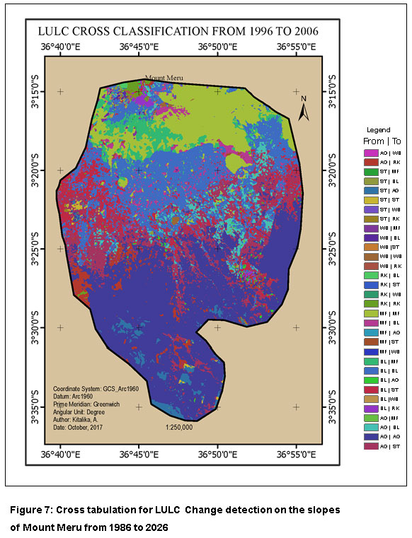 |
Figure 7: Cross tabulation for LULC Change detection on the slopes of Mount Meru from 1986 to 2026 |
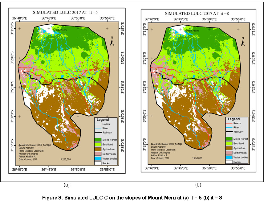 |
Figure 8: Simulated LULC C on the slopes of Mount Meru at (a) it = 5 (b) it = 8. Click here to view figure |
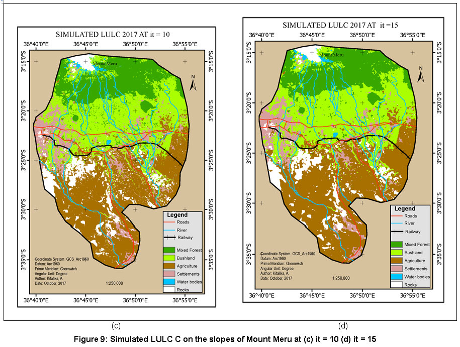 |
Figure 9: Simulated LULC C on the slopes of Mount Meru at (c) it = 10 (d) it = 15. Click here to view figure |
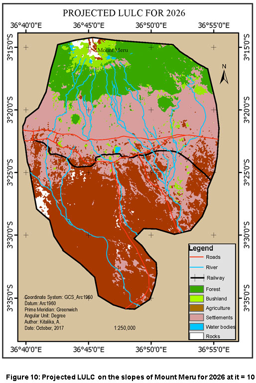 |
Figure 10: Projected LULC on the slopes of Mount Meru for 2026 at it = 10. Click here to view figure |
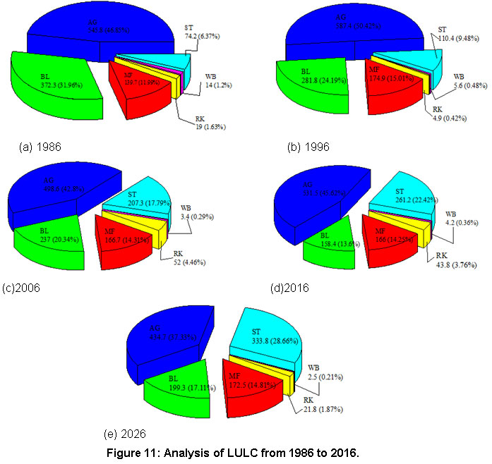 |
Figure 11: Analysis of LULC from 1986 to 2016. Click here to view figure |
Table 4: Actual LULC detection values and its projection from 1986 to 2026.
|
LULUC |
AREA (km2) |
|
NET GAIN AND LOSS (km2) |
NET GAIN AND LOSS (%) |
|||||||||||
|
1986 |
1996 |
2006 |
2016 |
2026* |
1996-1986 |
2006-1996 |
2016-2006 |
2016-1986 |
2026*-2016 |
1996-1986 |
2006-1996 |
2016-2006 |
2016-1986 |
2026*-2016 |
|
|
MF |
139.7 |
174.9 |
166.7 |
166.0 |
172.5 |
35.2 |
-8.2 |
-0.7 |
26.3 |
6.5 |
3.0 |
-0.7 |
-0.1 |
2.3 |
0.6 |
|
BL |
372.3 |
281.8 |
237.0 |
158.4 |
199.3 |
-90.5 |
-44.9 |
-78.5 |
-213.9 |
40.9 |
-7.8 |
-3.9 |
-6.7 |
-18.4 |
3.5 |
|
AG |
545.8 |
587.4 |
498.6 |
531.5 |
434.7 |
41.6 |
-88.8 |
32.9 |
-14.3 |
-96.7 |
3.6 |
-7.6 |
2.8 |
-1.2 |
-8.3 |
|
ST |
74.2 |
110.4 |
207.3 |
261.2 |
333.8 |
36.2 |
96.8 |
53.9 |
187.0 |
72.6 |
3.1 |
8.3 |
4.6 |
16.1 |
6.2 |
|
WB |
14.0 |
5.6 |
3.4 |
4.2 |
2.5 |
-8.4 |
-2.2 |
0.8 |
-9.8 |
-1.7 |
-0.7 |
-0.2 |
0.1 |
-0.8 |
-0.1 |
|
RK |
19.0 |
4.9 |
52.0 |
43.8 |
21.8 |
-14.1 |
47.1 |
-8.2 |
24.8 |
-22.0 |
-1.2 |
4.0 |
-0.7 |
2.1 |
-1.9 |
Table 5: Classification accuracy assessment for 2016 and other overall accuracy
|
LULC |
MF |
BL |
AG |
ST |
WB |
RK |
Total |
Accuracy (%) |
Overall Accuracy (%) |
||||
|
User's |
Producer's |
Year |
Total test points |
Correct points |
Accuracy |
||||||||
|
MF |
4 |
1 |
0 |
0 |
0 |
0 |
5 |
80 |
100 |
1986 |
25 |
20 |
80 |
|
BL |
0 |
4 |
1 |
0 |
0 |
0 |
5 |
80 |
80 |
1996 |
25 |
21 |
84 |
|
AG |
0 |
0 |
5 |
1 |
0 |
0 |
6 |
83 |
63 |
2006 |
25 |
20 |
80 |
|
ST |
0 |
0 |
1 |
6 |
0 |
0 |
7 |
86 |
75 |
2016 |
33 |
27 |
81.5 |
|
WB |
0 |
0 |
0 |
0 |
5 |
0 |
5 |
100 |
100 |
|
|
|
|
|
RK |
0 |
0 |
1 |
1 |
0 |
3 |
5 |
60 |
100 |
|
|
|
|
|
Total |
4 |
5 |
8 |
8 |
5 |
3 |
33 |
81.5 |
|
|
|
||
Table 6: Markov transition probability matrix 1996 to 2006
|
MF |
BL |
AG |
ST |
WB |
RK |
Model Validation |
||
|
MF |
0.7434 |
0.2178 |
0 |
0.032 |
0.003 |
0.004 |
Kstandard |
0.87 |
|
BL |
0.1243 |
0.5867 |
0 |
0.270 |
0.004 |
0.015 |
Kno |
0.88 |
|
AG |
0.0003 |
0.0638 |
0.7 |
0.192 |
0 |
0.057 |
Klocation |
0.91 |
|
ST |
0.0051 |
0 |
0.9 |
0.106 |
0.002 |
0.002 |
it |
10 |
|
WB |
0.3431 |
0.2284 |
0 |
0.014 |
0.303 |
0.112 |
||
|
RK |
0 |
0.2311 |
0 |
0.025 |
0.023 |
0.721 |
||
Table 7: Cross tabulation proportions of change
|
1986 |
Kappa Index (KIA) |
|||||||||
|
LULC |
MF |
BL |
AG |
ST |
WB |
RK |
Total |
1986 |
1996 |
|
|
1996 |
MF |
0.059 |
0.088 |
0.001 |
0.001 |
0.002 |
0.000 |
0.150 |
0.401 |
0.309 |
|
BL |
0.036 |
0.165 |
0.030 |
0.005 |
0.005 |
0.002 |
0.242 |
0.361 |
0.532 |
|
|
AG |
0.020 |
0.062 |
0.386 |
0.029 |
0.001 |
0.007 |
0.504 |
0.645 |
0.560 |
|
|
ST |
0.004 |
0.005 |
0.051 |
0.029 |
0.001 |
0.006 |
0.095 |
0.389 |
0.253 |
|
|
WB |
0.002 |
0.000 |
0.000 |
0.000 |
0.002 |
0.000 |
0.005 |
0.181 |
0.460 |
|
|
RK |
0.000 |
0.000 |
0.001 |
0.000 |
0.002 |
0.001 |
0.004 |
0.074 |
0.293 |
|
|
Total |
0.120 |
0.320 |
0.469 |
0.064 |
0.012 |
0.016 |
1.000 |
Overall |
0.459 |
|
|
1996 |
Kappa Index(KIA) |
|||||||||
|
LULC |
MF |
BL |
AG |
ST |
WB |
RK |
Total |
1996 |
2006 |
|
|
2006 |
MF |
0.102 |
0.037 |
0.002 |
0.001 |
0.002 |
0.000 |
0.143 |
0.627 |
0.663 |
|
BL |
0.038 |
0.123 |
0.039 |
0.002 |
0.001 |
0.001 |
0.203 |
0.383 |
0.478 |
|
|
AG |
0.001 |
0.013 |
0.336 |
0.078 |
0.000 |
0.000 |
0.428 |
0.417 |
0.567 |
|
|
ST |
0.008 |
0.063 |
0.094 |
0.012 |
0.000 |
0.000 |
0.178 |
-0.060 |
-0.029 |
|
|
WB |
0.001 |
0.001 |
0.000 |
0.000 |
0.001 |
0.000 |
0.003 |
0.227 |
0.372 |
|
|
RK |
0.001 |
0.005 |
0.034 |
0.002 |
0.001 |
0.003 |
0.045 |
0.626 |
0.056 |
|
|
Total |
0.150 |
0.242 |
0.504 |
0.095 |
0.005 |
0.004 |
1.000 |
Overall |
0.393 |
|
|
2006 |
Kappa Index (KIA) |
|||||||||
|
LULC |
MF |
BL |
AG |
ST |
WB |
RK |
Total |
2006 |
2016 |
|
|
2016 |
MF |
0.138 |
0.005 |
0.000 |
0.000 |
0.000 |
0.000 |
0.143 |
0.956 |
0.961 |
|
BL |
0.005 |
0.127 |
0.000 |
0.003 |
0.000 |
0.001 |
0.136 |
0.564 |
0.915 |
|
|
AG |
0.000 |
0.000 |
0.428 |
0.024 |
0.000 |
0.005 |
0.456 |
1.000 |
0.892 |
|
|
ST |
0.000 |
0.071 |
0.000 |
0.151 |
0.000 |
0.002 |
0.224 |
0.806 |
0.604 |
|
|
WB |
0.001 |
0.000 |
0.000 |
0.000 |
0.003 |
0.000 |
0.004 |
0.914 |
0.750 |
|
|
RK |
0.000 |
0.000 |
0.000 |
0.000 |
0.000 |
0.037 |
0.038 |
0.832 |
0.996 |
|
|
Total |
0.143 |
0.203 |
0.428 |
0.178 |
0.003 |
0.045 |
1.000 |
Overall |
0.837 |
|
|
1986 |
Kappa Index (KIA) |
|||||||||
|
LULC |
MF |
BL |
AG |
ST |
WB |
RK |
Total |
1986 |
2016 |
|
|
2016 |
MF |
0.061 |
0.078 |
0.001 |
0.001 |
0.002 |
0.000 |
0.143 |
0.425 |
0.349 |
|
BL |
0.024 |
0.085 |
0.018 |
0.004 |
0.005 |
0.001 |
0.136 |
0.150 |
0.446 |
|
|
AG |
0.017 |
0.038 |
0.347 |
0.043 |
0.001 |
0.010 |
0.456 |
0.522 |
0.549 |
|
|
ST |
0.016 |
0.117 |
0.078 |
0.012 |
0.001 |
0.001 |
0.224 |
-0.053 |
-0.013 |
|
|
WB |
0.001 |
0.000 |
0.000 |
0.000 |
0.002 |
0.000 |
0.004 |
0.159 |
0.540 |
|
|
RK |
0.001 |
0.001 |
0.025 |
0.004 |
0.002 |
0.004 |
0.038 |
0.223 |
0.095 |
|
|
Total |
0.001 |
0.320 |
0.469 |
0.064 |
0.012 |
0.016 |
1.000 |
Overall |
0.311 |
|
Table 8: Cross tabulation by quantitative change (km2)
|
1986 |
||||||||
|
LULUC |
MF |
BL |
AG |
ST |
WB |
RK |
Total |
|
|
1996 |
MF |
68.6 |
102.5 |
1.2 |
0.9 |
1.7 |
0.0 |
174.9 |
|
BL |
41.6 |
192.0 |
34.7 |
6.2 |
5.6 |
1.7 |
281.8 |
|
|
AG |
22.7 |
71.8 |
449.9 |
33.4 |
1.0 |
8.6 |
587.4 |
|
|
ST |
4.4 |
5.5 |
59.4 |
33.2 |
0.9 |
7.0 |
110.4 |
|
|
WB |
2.1 |
0.5 |
0.1 |
0.2 |
2.6 |
0.0 |
5.6 |
|
|
RK |
0.2 |
0.0 |
0.6 |
0.3 |
2.2 |
1.5 |
4.9 |
|
|
Total |
139.7 |
372.3 |
545.8 |
74.2 |
14.0 |
19.0 |
1165.0 |
|
|
1996 |
||||||||
|
LULUC |
MF |
BL |
AG |
ST |
WB |
RK |
Total |
|
|
2006 |
MF |
118.9 |
42.6 |
2.4 |
0.6 |
2.0 |
0.0 |
166.7 |
|
BL |
43.7 |
143.2 |
45.0 |
2.4 |
1.4 |
1.3 |
237.0 |
|
|
AG |
0.9 |
15.5 |
391.4 |
90.6 |
0.0 |
0.0 |
498.6 |
|
|
ST |
9.7 |
73.6 |
109.2 |
14.2 |
0.2 |
0.2 |
207.3 |
|
|
WB |
0.6 |
1.2 |
0.1 |
0.1 |
1.3 |
0.1 |
3.4 |
|
|
RK |
1.0 |
5.6 |
39.3 |
2.4 |
0.6 |
3.1 |
52.0 |
|
|
Total |
174.9 |
281.8 |
587.4 |
110.4 |
5.6 |
4.9 |
1165.0 |
|
|
2006 |
||||||||
|
LULUC |
MF |
BL |
AG |
ST |
WB |
RK |
Total |
|
|
2016 |
MF |
160.4 |
5.6 |
0.0 |
0.0 |
0.0 |
0.0 |
166.0 |
|
BL |
5.7 |
147.6 |
0.0 |
3.7 |
0.2 |
1.2 |
158.4 |
|
|
AG |
0.0 |
0.3 |
498.5 |
27.4 |
0.0 |
5.2 |
531.5 |
|
|
ST |
0.1 |
82.9 |
0.0 |
176.1 |
0.0 |
2.0 |
261.2 |
|
|
WB |
0.6 |
0.3 |
0.0 |
0.0 |
3.1 |
0.0 |
4.2 |
|
|
RK |
0.0 |
0.0 |
0.1 |
0.1 |
0.0 |
43.6 |
43.8 |
|
|
Total |
166.7 |
237.0 |
498.6 |
207.3 |
3.4 |
52.0 |
1165.0 |
|
|
1986 |
||||||||
|
LULUC |
MF |
BL |
AG |
ST |
WB |
RK |
Total |
|
|
2016 |
MF |
70.8 |
91.2 |
1.5 |
0.7 |
1.9 |
0.0 |
166.0 |
|
BL |
27.7 |
98.8 |
20.9 |
4.2 |
6.1 |
0.9 |
158.4 |
|
|
AG |
19.8 |
44.6 |
404.0 |
50.6 |
0.7 |
11.7 |
531.5 |
|
|
ST |
18.4 |
136.2 |
90.6 |
13.6 |
0.6 |
1.6 |
261.2 |
|
|
WB |
1.4 |
0.1 |
0.2 |
0.2 |
2.2 |
0.0 |
4.2 |
|
|
RK |
1.5 |
1.4 |
28.7 |
5.0 |
2.6 |
4.8 |
43.8 |
|
|
Total |
1.5 |
372.3 |
545.8 |
74.2 |
14.0 |
19.0 |
1165.0 |
|
Table 9: Position model validation for 2016
|
LULC |
MF |
BL |
AG |
ST |
WB |
RK |
Total |
Accuracy (%) |
|
MF |
7 |
1 |
0 |
0 |
0 |
0 |
8 |
87.5 |
|
BL |
0 |
6 |
1 |
1 |
0 |
0 |
8 |
75 |
|
AG |
0 |
1 |
6 |
1 |
0 |
0 |
8 |
75 |
|
ST |
0 |
0 |
0 |
7 |
0 |
1 |
8 |
87.5 |
|
WB |
0 |
0 |
0 |
0 |
8 |
0 |
8 |
100 |
|
RK |
0 |
0 |
1 |
1 |
0 |
4 |
6 |
66.7 |
|
Total |
7 |
8 |
8 |
10 |
8 |
5 |
46 |
82 |
Model Validation
It was necessary to validate the customized CA-Markov model and assess whether it could be used for simulation of the 10 years (2026) prediction LULC. The process was done through comparison of several simulated maps of 2006 at iteration 5, 8, 10 and 15 (Figure 8 and 9) with the actual LULC map of 2006 and assessment of their Kappa Indices (KIA) optimal values with their respective iterations. The validated model was observed at iteration 10 with satisfying required minimum value for model validation Kappa of 0.80 in which under this study Kstandard, Kno and Klocation of 0.87, 0.88 and 0.91 were obtained, respectively (Table 6) and therefore the model was adopted.47–50 Similar model validation for future land use in Tehran was done by Arsanjani et al., in their study and found that found strong correlation between the actual, map and predicted model map at Kstandard or 0.91 and Klocation of 0.97 at iterations 3000.10
Land-use Change Prediction
The validated model was executed to project the LULC for the next 10 years (2026). The process was done together with the 2006 land-use map, the 1996–2006 transition area matrixes, as well as the 2006 transition potential maps. The resulting values for various land use changes are summarized in Table 4 and Figure 11. From figure 11(e) it is seen that the total land for agriculture (AG) will decrease by 8.29% which will be replaced by human settlement (ST) and bush land (BL) which will also increase by 6.2% and 3.51% by 2026, respectively. It is obvious that the increased human settlement will be caused by increased population which is among the expected major land use change for urbanization process of an area. It is also anticipated that in the next 10 years there will be a very little increase of mixed forest (MF) by 0.56% which is a good sign of good forest conservation strategy by the government. It should be noted that the increase in urbanization process normally is associated with increase in demand of land for construction which can involve clearance of natural resources in some conserved areas such as forest and water which in this study if the present government laws and rules will continue to be strictly followed the conserved forest will continue to survive. Also the status of water body will be in a bad situation in relation to increased population since the demand for fresh water will be high if no other water sources will be invented. The study shows decrease in fresh water bodies (WB) by 0.15% from 2016 to 2026 which is highly alarming for comfortable resulting urban area. In addition, the area covered by rocks will decrease in the next 10 years by1.89% which will mostly be expected to be converted into settlements due to the fact that there is minimum possibility of areas covered with rocks to be converted in any of the remaining land use categories.
Despite the anticipated land use changes expected to occur in the next 10 years, some challenges occurred in the process of image and land use classifications hence in the projecting model. For example, the study area has rocks on the mountain peak and other areas which its reflectance somehow resembled that of iron and white plastic sheets and plastic covering the buildings and several other greenhouses in the flower farms. This must have led some confusion for actual land use category classification. It is unfortunate that the most common worldwide method for validation of the projected LULC map saves to use the validated model at stated three (3) Kappa values as stated at model validation section. On the other side, comparison between the projected and real image after the specified time lapse can also be used to observe what has happened in real environment. The second alternative is worthless since the aim of projecting the future LULC change of environment resides on protecting them from alarming current observed changes. However, there are some features which are necessary in any correct mapping process, such as scale and location which are sensitive to any feature presentations.51,52 In this study, this feature has been taken care of by assuring similar scale has been used for all analysis images through windowing and correct georeferencing is done in addition to inspection for correct LULC classification in comparison with simulated and real map. Difficulties appear in validation of simulated and projected maps since there are no true references as there is inexistence. Therefore, the best validation method in this study was designed in order to ensure that the model predicted reasonably, the locations and land use of the predicted cells for development and assessed their feasibilities in comparison to the real map.10 Comparison was done with true features based on the predictor model map of 2006 in relation to the true map of the same year and their outcomes were as summarized in Table 9. From the table the comparison showed correctness by 82% which can also account for similar percentage correctness of the project LULC map for 2026.
LULC and Discharge
A study was done to evaluate whether there is any effect on change of canopy cover in relation to river discharge when other parameters remained constant. The analysis shows that there was very weak correlation between the two (r ≤ 0.3, n = 4, p ≤ 0.03, Figure 12). These results suggest that the presence of good canopy cover feature around any catchment area is not the only cause for maximized recharge potential of any watershed rather it can add potentials for long term discharge and recharge of the river. Therefore, a combination of factors such as soil structure and texture, terrain and weather conditions of a place may account in addition to canopy cover. Further analyses were needed to find out other contributing factors for discharge potentials of the river whereby the correlation analysis was done between precipitations of an area in relation to the discharge patterns of rivers for thirty (30) years in ten (10) years intervals. The analysis showed that there is a strong positive correlation between the two [(a) r = 0.99, n = 4, p ≤ 0.003, (b) r = 0.97, n = 4, p ≤ 0.01 (c) r = 0.88, n = 4, p ≤ 0.05, (d) r = 0.93, n = 4, p ≤ 0.04), Figure 13 and 14)] suggesting that the main water sources from rivers is precipitation. While this positive correlation is promising for the two relationships it should be remembered that the feasibility of the holding capacity of precipitated water is much more pronounced when there is good canopy cover of an area in order to minimize the runoff, evaporation and increase the soil holding capacity for water and porous aquifers which in turn will give a good recharge potential of any watershed. It should also be made clear that this assessment was done in the assumption that other confounding factors for discharge such as soil type, water, agriculture and transpiration (SWAT) remained constant throughout the year otherwise the analysis could be invalid. It should be noted that most rivers from this study area originates from the top hills of mount Meru which the LULC study shows that water bodies from the mountain peak have been decreasing continuously from 1986 to 2016 (Figure 3 and Table 3 ). These calls upon Tanzanian country and the world as a whole to put in place all necessary environmental protection practices such as reducing the greenhouse gases emission which are the main cause of the global climate change such as increase in atmospheric temperature which has accelerated the melting of ice caps all over the world including Mount Meru which is within the study area.
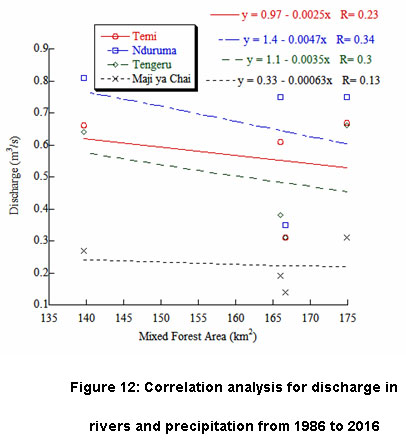 |
Figure 12: Correlation analysis for discharge in rivers and precipitation from 1986 to 2016 |
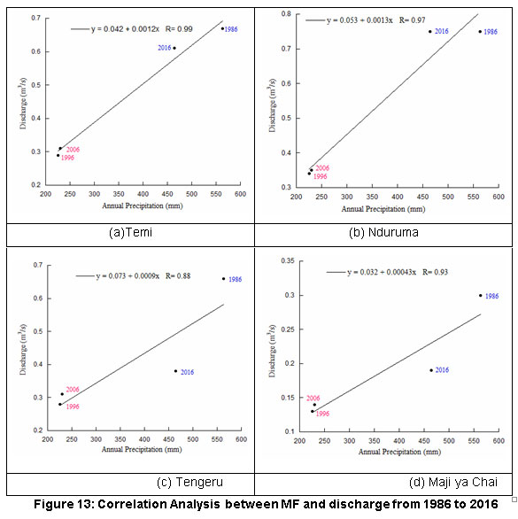 |
Figure 13: Correlation Analysis between MF and discharge from 1986 to 2016 Click here to view figure |
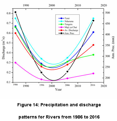 |
Figure 14: Precipitation and discharge patterns for Rivers from 1986 to 2016 |
In addition, the analysis from Figure 14 indicates that Temi and Nduruma Rivers had almost similar and higher discharge pattern and levels compared to Tengeru and Maji ya Chai Rivers. Despite such similarity, the discharge capacity of Nduruma goes down during the dry season due to high water abstraction by AWSA in the season which is further accelerated by the irrigation practices in the downstream. A combination of two factors have caused drying off of the river in the floodplain area specifically during the dry season hence causing massive deaths of aquatic creatures and the riparian vegetations.
Conclusion
This study indicates a significant land use changes of the area which might have caused even changes in other environmental parameters such as the natural vegetation cover, living organisms, and water characteristics. The study has shown a rapid conversion of bush and agriculture land into human settlement which is likely to be a common case for any area in transition into urbanization. However, the challenge arises when the increases human settlements which reflect increasing in human population are at the expense of reduced agriculture land (AG). That means while the population is increasing, the capacity to be fed by the same environment is minimized meaning that the sustainability of such urban population must involve importation of food and food products from others areas which will eventually increase the living cost. In addition, the present study has assessed the LULC of the area using only the features presented in the satellite images which are the outcomes of the influencing factors. Such factors which can affect the environment include social, political, scientific, technological, socioeconomically and biophysical factors which if they could be integrated in the CA-Markov model, could improve the accuracy of simulation thus giving the actual situation of the land use change which could be higher than 82% accurate. Furthermore, errors must have happened in rock classification since in the study area there are greenhouses and roads which could show similar reflectance with the rocks and therefore some of the classification could have included in either settlements or rocks. Such errors may account for the 18% inaccuracy. Lastly, the observed continuous land use changes in the area attracts attention to further studies of other associated environmental features which are also likely to have been affected.
Acknowledgments
The authors are grateful to Tanzania Government and the Dar es Salaam University College of Education (DUCE) for financing this study and the VLIR-UOS project for providing some laboratory instruments and transport in the entire study.
References
- Noe C. The Dynamics of Land Use Changes and Their Impacts on the Wildlife Corridor between Mt . Kilimanjaro and Amboseli National Park , Dar es Salaam, Tanzania. 2003.
- Lambin E. F., Turner B. L., Geist H. J., Agbola S. B., Angelsen A., Bruce J. W., Xu J.The Causes of Land-use and Land-cover Change: Moving Beyond the Myths. Global Environmental Change. 2001;11(4):261-269.
CrossRef - Richter S., Postel B. Rivers for Life: Managing Water for People and Nature, Island Press, Washington D.C. 2003.
- The International Bank for Reconstruction and Development/ The World Bank. Water Resources and Environment Technical Note C1. Environmental Flows: (Richard Davis RH, ed.), Washngton D.C. 2003.
- Bisht B. S., Tiwari P. C. Land-use Planning for Sustainable Resource Development in Kumaun Lesser Himlalaya, A Study of the Gomli Watershed. International Journal of Sustainable Development and World Ecology. 1996;3(4):23-34.
CrossRef - Mbonile M. J. Population, Migration, and Water Conflicts in the Pangani River Basin, Tanzania. 2006.
- Tu M. Assessment of the Effects of Climate Variability and Land Use Change on the Hydrology of the Meuse River Basin, A.A. Balkema Publishers, Oxfordshire. 2006.
- Notter B., Hurni H., Wiesmann U., Ngana J. O. Evaluating Watershed Service Availability Under Future Management and Climate Change Scenarios in the Pangani Basin. Physics and Chemistry of Earth. 2013;61-62:1-11.
CrossRef - Subedi P., Subedi K., Thapa B. Application of a Hybrid Cellular Automaton – Markov ( CA-Markov ) Model in Land-Use Change Prediction : A Case Study of Saddle Creek Drainage Basin , Florida. Applied Ecology and Environmental Science. 2013;1(6):126-132.
CrossRef - Arsanjani J. J., Kainz W., Mousiv A. J. Tracking Dynamic Land-use Change Using Spatially Explicit Markov Chain Based on Cellular Automata : The Case of Tehran. International Journal of Image and Data Fusion. 2011;2(4):329-345.
CrossRef - Verburg P. H., Overmars K. P., Huigen M. G. A., Groot WT De., Veldkamp A. Analysis of the Effects of Land Use Change on Protected Areas in the Philippines. Applied Geography. 2006;26:153-173.
CrossRef - Water and Nature Initiative, Pangani River Basin Flow Assessment Scenario Report, International Union for Conservation of Nature and Pangani Basin Water Board Pangani Basin Water Office (IUCN-PBWO), Moshi, Tanzania. 2010;295.
- Turpie J. K., Ngaga Y. M., Karanja F. Catchment Ecosystems and Downstream Water : International Union for Conservation of Nature (IUCN). 2005.
- Lalika M. C. S., Meire P., Ngaga Y. M., Chang’a L. Understanding watershed Dynamics and Impacts of Climate Change and Variability in the Pangani River Basin , Tanzania. Ecohydrology and Hydrobiology. 2014;67:1-13.
- International Encyclopedia of Huma Geography. In: International Encyclopedia of Huma Geography. 8th ed. Elservier. 603;2009.
- Houet T., Hubert-moy L., Houet T., Modeling L. H., States F. Modeling and Projecting Land-Use and Land-Cover Changes with Cellular Automaton in Considering Landscape Trajectories. Europian Association of Remote Sensing Laboratory. 2007;5(1):63-76.
- Singh A. Digital Change Detection Techniques Using Remotely-Sensed Data. International Journal of Remote Sensing. 2010;10(6):989-1003.
CrossRef - Marko K., Zulkarnain F., Kusratmoko E. Coupling of Markov Chains and Cellular Automata Spatial Models to Predict Land Cover Changes ( Case Study : Upper Ci Leungsi Catchment Area ), Earth and Environmental Science. 2016;47(012032).
- Behera M. D., Borate S. N., Panda S. N. Modelling and Analyzing the Watershed Dynamics Using Cellular Automata ( CA )– Markov Model – A Geo-Information Based Approach. Journal of Earth System and Science. 2012;121(4):1011-1024.
CrossRef - Yu-Pin L., Yun-Bin L., Wang Y., Hong N. Monitoring and Predicting Land-use Changes and the Hydrology of the Urbanized Paochiao Watershed in Taiwan Using Remote Sensing Data, Urban Growth Models and a Hydrological Model, Sensors. 2008;8:658-680.
CrossRef - Shively G., Coxhead I. Conducting Economic Policy Analysis at A Landscape Scale : Examples from a Philippine Watershed. Agriculture Ecosystem and Environment.. 2004;104:159-170.
CrossRef - Kundu PM, Olang LO. The Impact Of Land Use Change on Runoff and Peak Flood Discharges for the Nyando River in Lake Victoria Drainage Basin, Kenya. Water and Society. 2011;153:83-94.
- Mulubrehan K. H. Analysing the Effect of Land Cover Change on Catchment Discharge. Tigray. 2014.
- Schilling K. E., Jha M. K., Zhang Y., Gassman P. W. Impact of Land Use and Land Cover Change on the Water Balance of a Large Agricultural Watershed : Historical Effects and Future Directions Impact of Land Use And Land Cover Change on The Water Balance of a Large Agricultural Watershed : Historical Effects. Water Resources Research. 2016;44(W00A09).
- Heil M. Effects of Large-Scale Changes in Land Cover on the Discharge of the Tocantins River , Southeastern Amazonia. Journal of Hydrology. 2003;283:206-217.
CrossRef - Cristina L., Dias P., Macedo M. N., Heil M., Coe M. T., Neill C. Effects of Land Cover Change on Evapotranspiration and Streamflow of Small Catchments in the Upper Xingu River Basin , Central Brazil. Journal of Hydrology:Regional Studies. 2015;4:108-122.
- Batty M. Modeling and Simulation in Geographic Information Science: Integrated Models and Grand Challenges. Procedia Social and Behaviour Sciences. 2011;21:10-17.
CrossRef - Neumann J. The general and Logical Theory of Automata. Cerebral mechanisms in behavior; the Hixon Symposium. 1951;10(3):1-41.
- Moreno N., Wang F., Marceau D. J. Implementation of a Dynamic Neighborhood in a Land-Use Vector-Based Cellular Automata Model. Computer Environment and Urban Systems. 2009;33(1):44-54.
​​​​​CrossRef - Benenson I., Torrens P. M. Geosimulation: Object-Based Modeling of Urban Phenomena. Computer Environment and Urban Systems t. 2004;28(1-2):1-8.
- de Almeida C. M., Batty M., Monteiro A. M. V., Filho G. S., Cerqueira B. S., Pennachin G. C., Lopes C. Stochastic Cellular Automata Modeling of Urban Land Use Dynamics: Empirical Development and Estimation. Computer Environment and Urban Systems. 2003;27(5):481-509.
​​​​​​​CrossRef - Syphard A. D., Clarke K. C., Franklin J. Using a Cellular Automaton Model To Forecast The Effects of Urban Growth on Habitat Pattern in Southern California. Complexity. 2005;2:185-203.
​​​​​​​CrossRef - Kamusoko C., Aniya M., Adi B., Manjoro M. Rural Sustainability Under Threat in Zimbabwe - Simulation of Future Land Use/Cover Changes in the Bindura District Based on the Markov-Cellular Automata Model. Applied Geography. 2009;29(3):435-447.
​​​​​​​CrossRef - Sinha S., Das S., Sahoo S. Geology & Geophysics Application of Markov Chain and Entropy Function for Cyclicity Analysis of a Lithostratigraphic Sequence - A Case History from the Kolhan Basin. Journal of Geology and Geophysics. 2015;4(5):224.
- Maarel E. V. D. Vegetation dynamics and dynamic vegetation. Acta Botanica Neerlandica. 1996;45(4):421-442.
​​​​​​​CrossRef - Muller M. R., Middleton J. A Markov Model of Land-Use Change Dynamics in the Niagara Region, Ontario, Canada. Landscape Ecology. 1994;9(2):151-157.
- Omidipoor M., Samani N. N., Change L., Filter S. Impact of Spatial Filter on Land-Use Changes Modelling Using Urban Cellular Automata. The International Archives of the Photogrammetry, Remote Sensing and Spatial Information Sciences. 2017;42-4/W4:7-10.
​​​​​​​CrossRef - Yang Y., Zhang S., Yang J., Xing X., Wang D. Using a Cellular Automata-Markov Model to Reconstruct Spatial Land-Use Patterns in Zhenlai County, Northeast China. Energies. 2015;8:3882-3902.
​​​​​​​CrossRef - Deep S. Urban Sprawl Modeling Using Cellular Automata. Egypt Journal of Remote Sensing and Space Sciences. 2014;17(2):179-187.
​​​​​​​CrossRef - Aithal B. H., Vinay S., Ramachandra T. V., Area S. Landscape Dynamics Modelling Through Integrated Markov, Fuzzy-AHP and Cellular Automata. IGARSS. 2014;978-1-4799:3160-3163.
- Kitalika A. J., Machunda R. L., Komakech H. C., Njau K. N. Fluoride variations in rivers on the slopes of mount meru in Tanzania. Journal of Chemistry. 2018;2018(7140902):18.
​​​​​​​CrossRef - UNDP. Arusha Region Water Master Plan, Final Report. 2000.
- Gea F. Analysis of Issues Connected with Water Supplying in Maasai Pasturelands Around the Village of Uwiro (Arusha, Tanzania). 2005.
- Kitalika A. J., Machunda R. L., Komakech H. C., Njau K. N. Physicochemical and Microbiological Variations in Rivers on the Foothills of Mount Meru, Tanzania. International Journal of Scientific and Engineering Reserch. 2017;8(9):1320-1346.
​​​​​​​CrossRef - Coppin POLR., Bauer M. E., Bauer M. E. Change Detection in Forest Ecosystems with Remote Sensing Digital Imagery Digital Change Detection in Temperate Forests. Remote Sensing Review. 1996;13:207-234.
​​​​​​​CrossRef - Kashaigili J. J., Mbilinyi B. P., Mccartney M., Mwanuzi F. L. Dynamics of Usangu Plains Wetlands : Use of Remote Sensing and GIS as Management Decision Tools. Physics and Chemistry of Earth. 2006;31:967-975.
​​​​​​​CrossRef - Pontius R. Modeling Tropica1 Land Use Change and Assessing Policies to Reduce Carbon Dioxide Release from Africa, Graduate Program in Environmental Science. SUNY-ESF, Syracuse, New York. 1994.
- Pontius Jr R., Suedmeyer B. Components of Agreement in Categorical Maps at Multiple Resolutions. In: Lyon RSL and JG, ed. Remote Sensing and GIS Accuracy Assessment. Boca Raton FL. 233-251;2004).
- Pontius Jr R., Gil R. Statistical Methods to Partition Effects of Quantity and Location During Comparison of Categorical Maps at Multiple Resolutions. Photogrammetric Engineering & Remote Sensing. 2002;68(10):1041-10
- Pontius Jr R., Gil R. Quantification Error Versus Location Error in Comparison of Categorical Maps. Photogrammetric Engineering & Remote Sensing. 2000;66(8):1011-1016.
- Pontius Jr R. G., Huffaker D., Denman K. Useful Techniques of Validation for Spatially Explicit Land-Change Models. Ecological Modelling. 2004;179(4):45–461.
​​​​​​​CrossRef - Pontius Jr R. G., Shusas E., McEachern M. Detecting Important Categorical Land Changes While Accounting for Persistence. Agriculture Ecosystems and Environment. 2004;101(2–3):251–268.
​​​​​​​CrossRef


