Current World Environment

Introduction

The natural as well as socioeconomic variability of state Rajasthan which includes water resource management, agriculture, forestry, tourism etc. are highly influenced by a key component of hydrological cycle i.e. precipitation. Therefore, it is necessitated for predicting future precipitation change since it is an input for climate impact model to assess the consequences of global change in the climate. GCMs under climate input model often found inadequate due to the limited depiction of mesoscale atmospheric processes, topography and sea distribution. Besides, with respect to precipitation, GCMs show higher spatial scale (grid point area) compare to require in climate impact model and ultimately it will lead to in frequency statistics like exceedance of heavy precipitation.

As the response from the state control board, though several studies, Rajasthan is more likely to face the problem of increased water scarcity because of an overall decrease in rainfall and augmented evapotranspiration as a result of global warming. During the year, 1988, 1998, 1999, 2000 and 2001, Rajasthan has faced the drought-like situation. In addition, this state also has maximum susceptibility and lowest adaptive capacity fluctuating climate. Drought is frequent in a state like Rajasthan and intensity of droughts will determine the condition of the state, in terms of its natural and socioeconomic studies. Evapotranspiration can be increased by even one per cent increased the temperature from base data. Therefore, the quality and quantity of surface and groundwater resources of Rajasthan are drastically deteriorated in the last twenty years.

Material and Method

Study Area

In terms of area, Rajasthan is the largest state in the country occupying 3,42,000 square kilometres area. It has 33 districts and situated between 69°30' to 78°17'E longitude and 23^°30^'to 30^°12^' N latitude. The climate of Rajasthan in northwestern India is usually arid to semi-arid with hot temperatures over the year with extreme temperatures in both summer and winter. The state has two different epoch of rainfall, one is due to the South-West Monsoon after summer and another rainfall due to Western Disturbances.
 

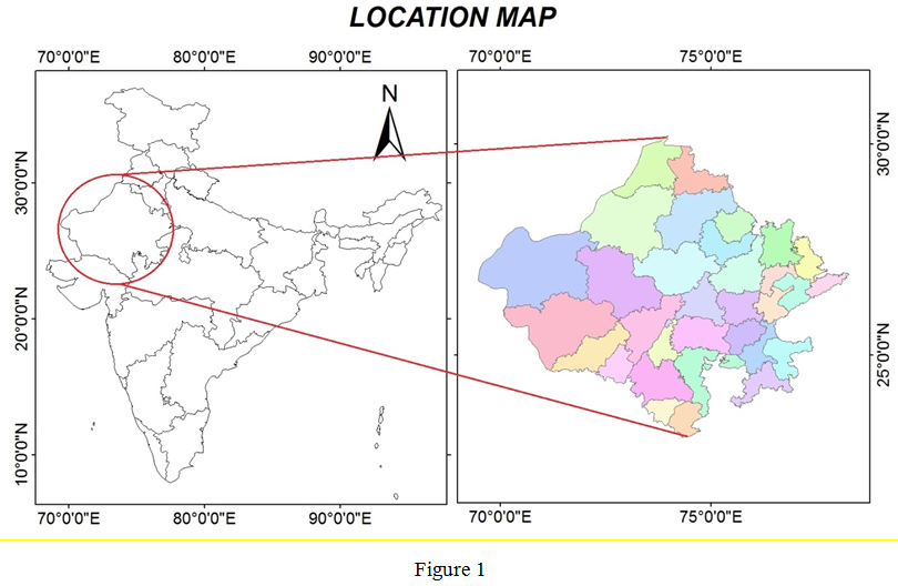Figure 1 Click here to view figure

Multiple Linear Regressions

MLR model is used to build the linear relationship between the dependent variable (predictand) and one or more than one independent variables (predictor). This method allows the prediction of a single predictand variable from a set of predictors variables.

The equation of MLR represents as: 



Formula 1

Where, Y^MLR = Estimated predictand (rainfall); α =Intercept; β =Regression coefficients; X = Predictors (26 predictors) which varies up to suitable n^th terms and  δ = error term.

Multiple linear regression attendant or observed a best-fit plane. It was evaluated with R². As a response to correlation coefficient (R) expresses the degree to which two or more predictors are related to the predictand.

Using the proposed methodology and The Pearson correlation coefficients amongst possible predictors as well as the recorded monthly precipitation were premeditated each time part and the entire period, at all grid points in the atmospheric province.

In the study 26 NCEP variables give in table 1, that is used by means of substitution of the recent opinion of GCM variables, and they were composed of the website of the Canadian Climate Change Scenarios Network (CCCSN) and it used in place of predictors in the downscaling model. There are no general rules for the selection of predictors but few researchers suggested that the way to choose an appropriate NCEP predictor. Selection of predictors differ from single province to others and mostly be contingent on the physiognomies of large-scale atmospheric circulation, seasonality, regional topography, and the predictand to be downscaled. The aerial scope of the climatic province has used the assortment of predictors is frequently selected which depend on the mechanism of rainfall in an extent.

Table 1: NCEP variables used by the select predictors for downscaling rainfall.

Estimation of Performance Downscaling Model

Downscaling model performance was evaluated on the basis of comparison between mean, variance and quartiles(25^th, 50^th, and 75^th) of observed and downscaled values of precipitation during both calibration and validation of the model. Various statistical parameters like RMSE, R², NSE were utilized to show the efficiency of the downscale model. The most widely used statistical parameter was selected for assessing the efficiency of the downscaled model.

Generally, a higher value of NSand CC indicates well correctness of model prediction whereas the lesser value of NS shows a poor model prediction. Nash-Sutcliffe ranges from - ∞ to 1. The value of NS = 1 shows a faultless match among the model and annotations, Whereas the efficiency of 0 shows that the model forecasts are as precise as the mean of the detected data. if value of efficiency is less than zero (- ∞ < E < 0) then detected mean is a superior predictor than the model.

Lesser valves of RMSE and NMSE during model calibration and validation gives smaller discrepancy among observed and predicted time series, therefore provide high accuracy in prediction. The correlation coefficient value can range from -1.00 to +1.00 where negative range shows the negative correlation while positive ranges show a positive correlation. The correlation coefficient value “1” shows the perfect correlation while “0” shows there is no correlation.

Results and Discussion

Development of Downscaled MLR model for prediction of rainfall

Model’s Calibration and Validation

The NCEP predictors used for MLR model calibration for epoch1961-1990 and validated for period 1991-2001 in contradiction of the experiential rainfall. Data of 30 years(1961-1990 ) used as a baseline due to availability of adequate period which is required to establish a reliable climatology, to include resilient global change signal. Calibration and validation were done separately for all the districts under study.

Predictors Selection

In this research, the selection of predictors has been considered using the cross-correlation technique. About ten parameters i.e., Mean sea level pressure, Surface wind direction, Surface divergence, 500 hPa airflow strength, 500 hPa zonal velocity, 500 hPavorticity, 500 hPa wind direction, 850 hPa geopotential height, Relative humidity at 500 hPa and Surface specific humidity were commonly used for all the 32 districts. However, out of these, the ten predictors about 4-6 parameters showed a strong correlation among the predictand and predictors for each district. Both positive, as well as negative correlation, has also been considered for estimation of downscaled rainfall.

Standardization and Validation of Downscaling Model

As per the assortment of predictors and predictands, The MLR was applied for every district to downscale rainfall. MLR model was based on regression coefficients, intercepts and error term, which depends upon the relationship between selected predictors and predictand. The performance of the downscaled model was judged on the basis of comparison between various statistical parameters like RMSE, NMSE, NASH and CC of detected and modelled precipitation during standardization and validation of the model. The observed result during the study was shown in table 2.

Table 2: Results for accuracy assessment during the calibration and validation for monthly rainfall time series in different location of Rajasthan.

The calibration, results of correlation coefficients for all the districts were found to be more than 0.8, which indicate a good correlation between observed and modelled rainfall. The validation of the correlation coefficient gave good result and it more than 0.68 for all the districts showing a good correlation between observed and modelled rainfall. The NMSE in the case of calibration and validation of MLR downscaling models range from 0.02 to 0.39 and 0.01 to 0.41 respectively, which is indicate less discrepancy between observed and predicted time series. Further, NASH efficiency for both calibration and validation period is about 0.60-0.97 and 0.50-0.98 respectively. The overall model results indicate good performance during calibration as well as validation using NCEP variables.

The calculation of downscaling model performance was done because of the comparison between mean and variance values of both experiential and modelled precipitation throughout and ardization and validation of the model, outcomes are shown in Table 3. The coefficient of variation between detected and modelled rainfall of downscaled model for all districts was ranged from 0.34 to 1.89, 0.34 to 1.35 for model calibration respectively, which clearly indicate that the downscaling model indicates that the downscaled model has predicted the observed precipitation with high accuracy during calibration of the model. Similarly results during model validation also, the coefficient of variation in the observed and modelled precipitation of downscaling model of all the districts range from 0.34  to 1.92 and 0.33 to 1.45 indicating a good match between the observed and modelled precipitation. However, it has been found that precipitation is minute over or under-predicted in approximate districts during model validation. For specimen, at Chittorgarh district, the detected precipitation was 68.22 mm whereas the model produces 66.69 mm.

Table 3: Mean and coefficient of variation for observed and modelled precipitation during model calibration and validation.

The observed precipitation variance was much higher than the simulated precipitation variance. Therefore, downscaled models were failed to capture the full spectrum of precipitation variance. The outcome of this study also revealed that the performance of downscaled models was not much efficient in arresting mean precipitation. But, the model was quite compatible to arrest variance in most of the districts. E.g. least variance of 0.34 and 0.33 was obtained in the observed and downscaled precipitation, respectively at Swaimadhopur district and in other districts also the appendix-I differences were not large throughout model calibration and validation.

Time Series Analysis of Detected and Downscaled Rainfall

Based on the comparison between the monthly time series of detected and downscaled precipitation, the efficacy of downscaled model during calibration and validation was estimated. This comparison was done for all districts under study individually. The result was shown in table 2 for all districts. Results describe that the monthly precipitation follows the analogous pattern like the detected precipitation. In limited districts, some months consume extreme precipitation standards, which remained under-predicted by the model. The extreme measures occurrences are a common phenomenon in hydrology, which frequently cannot be estimated with NCEP predictors. Testified that the downscaling model flops arrest the extreme precipitation. However, it can successfully arrest the mean. The model used in this study was observed to capture the mean and low precipitation more accurately.

Projection of Monthly Rainfall using HadCM3 (A2 & B2 Scenario)

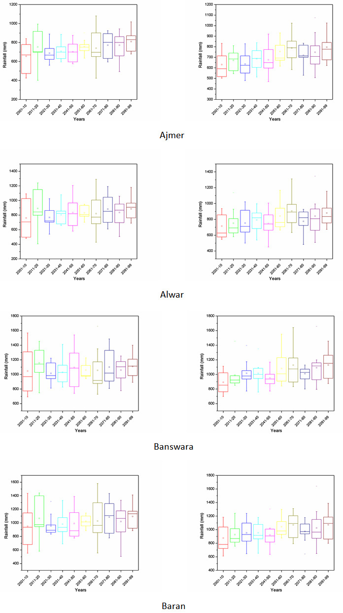
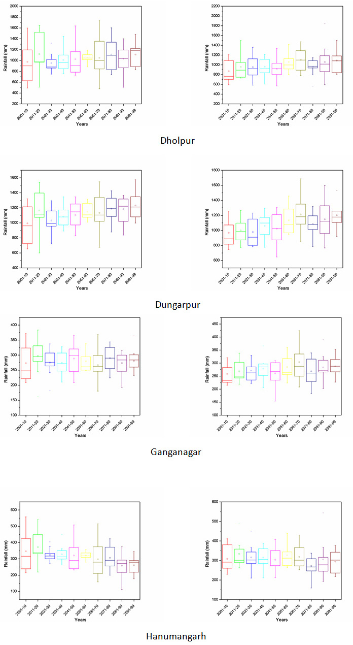
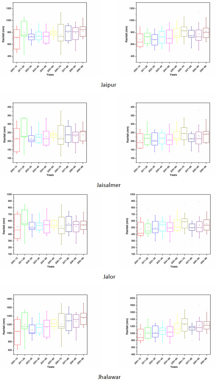
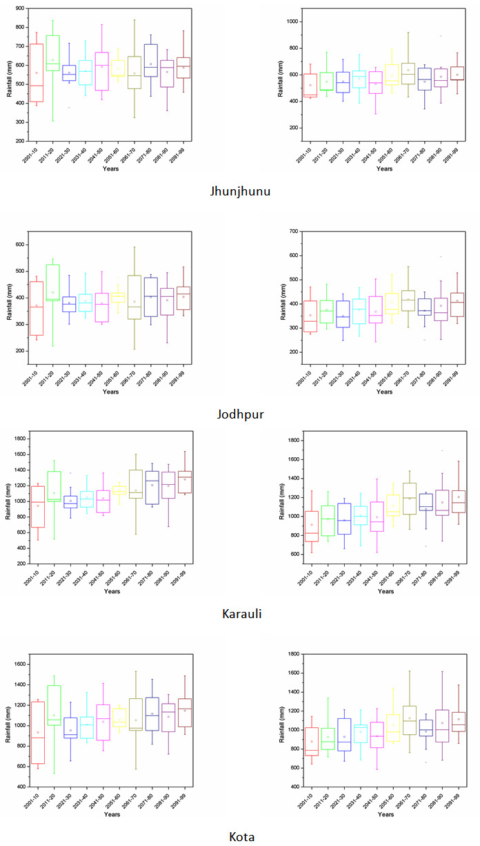
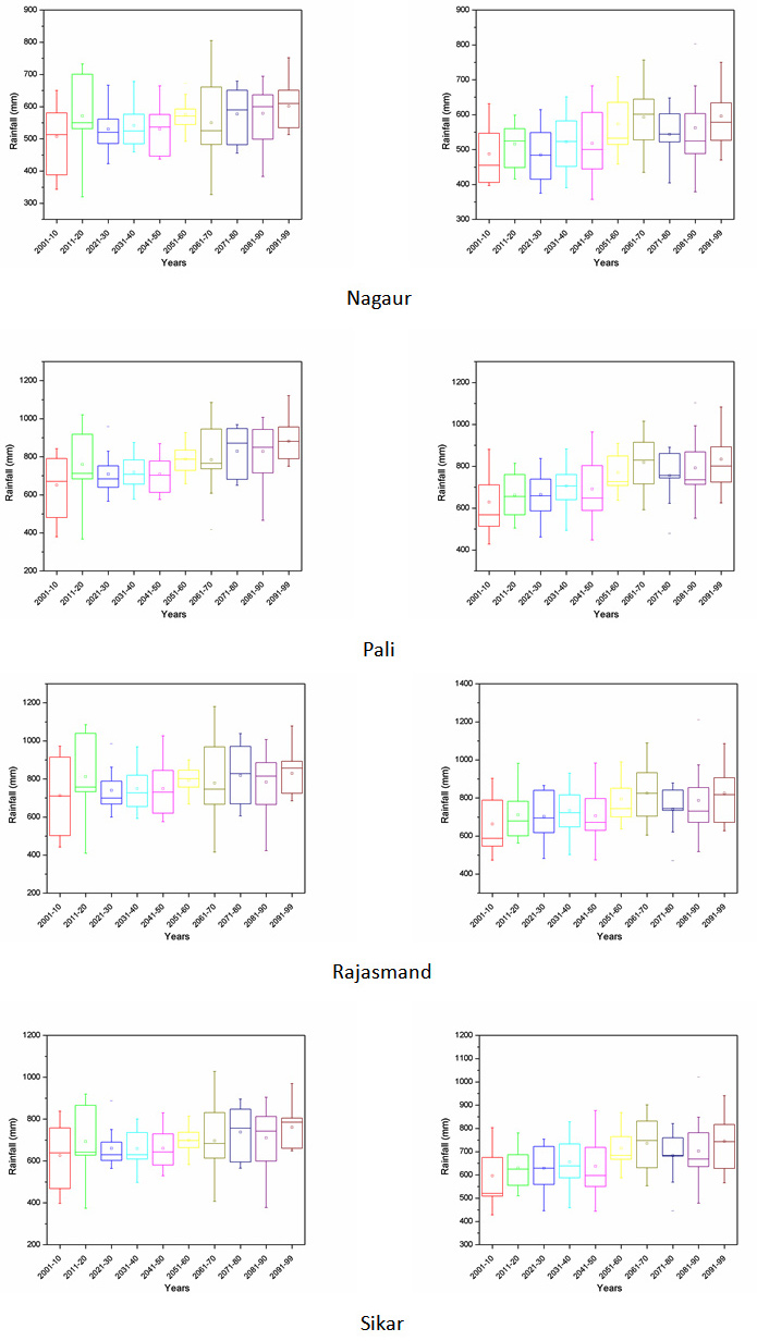
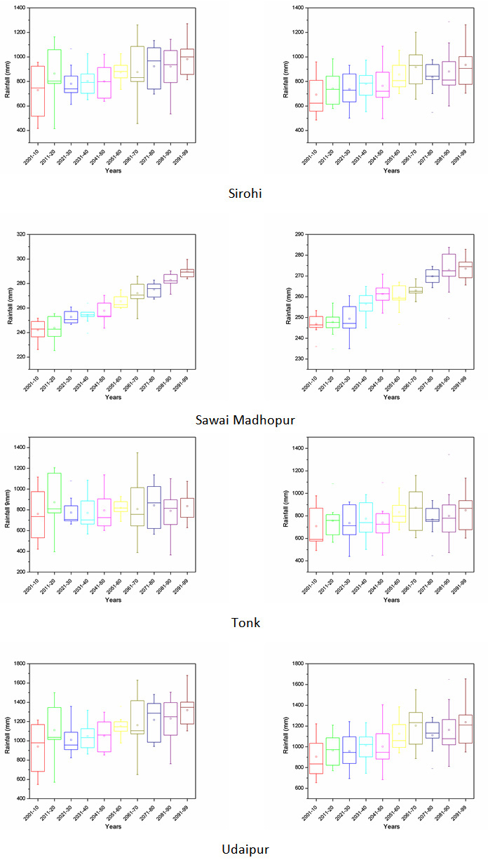
Projection of future scenarios has been carried out using the HadCM3 A2 & B2 emission scenarios with selected predictors. However, MLR downscaling techniques have been utilized for future projection of predictand. Further, a whole time series of monthly predictand has been divided into decadal form (10-year time scale) for better representation of results. Box plot of decadal time steps is used for the determination of pattern in predictand. The projected rainfall of all district for decadal periods of 2001-2010, 2011-2020, 2021-2030, 2031-2040, 2041-2050, 2051-2060, 2061-2070, 2071-2080, 2081-2090 and 2091-2099 are Appendix II. The box middle line showed median valves whereas upper and lower edges give the 75 per and 25 per of datasets respectively. The difference between 75 per and 25 per called interquartile range (IQR). The box plot of rainfall shows the increase in future rainfall in both cases of A2 and B2 scenarios for whole Rajasthan.

Conclusion

The native hydrological regimes of the arid and semi-arid regions are highly prejudiced by the changes in climatic variables. Therefore, it remains very much imperative to comprehend and model the influence of climate change over arid and semi-arid region under current and future scenario. A Multiple Linear Regression (MLR) model was used in the study to downscale the precipitation in data scarce arid and semi-arid regions of Rajasthan state of India, which considered as most susceptible areas to climate change. The dataset of NCEP reanalysis from twenty grid points which surrounds the study range was used to select the predictors based on principal component analysis (PCA). The data of monthly rainfall from 1961-1990 time periods were used for calibration as well as from 1991-2001 time period for authentication of the MLR model.

Performance of the MLR model to downscale monthly rainfall of Rajasthan was assessed to evaluate the climate change impact. The study showed that the MLR model is more superior to downscale precipitation in most districts under study area. Statistical downscaling of rainfall is quite difficult as a result of an erratic pattern of rainfall, poor relation local rainfall and ocean-atmospheric circulation parameters of arid regions. The outcome of the present study indicates that MLR could be used for downscaling of monthly rainfall of regions under arid and semi-arid. The result observed that the downscaling of rainfall showed an increase in future rainfall for both A2 and B2 scenario.

Acknowledgements

Thankful to both National Institute of Hydrology, Roorkee, Uttarakhand for providing essential data and Maps for my research work and Department of Farm Engineering, IAS, Banaras Hindu University, Varanasi for referring me to National Institute of Hydrology, Roorkee for my research work.

References

1. Cohen SJ Bringing the global warming issue closer to home: the challenge of regional impact studies. Bull Am MeteorolSoc 1990; 71:520–526.
   CrossRef
2. Von Storch, H., Zorita, E., & Cubasch, U. Downscaling of global climate change estimates to regional scales: an application to Iberian rainfall in wintertime. Journal of Climate 1993; 6(6): 1161-1171.
   CrossRef
3. Schmidli, J., Goodess, C. M., Frei, C., Haylock, M. R., Hundecha, Y., Ribalaygua, J., & amp; Schmith, T. Statistical and dynamical downscaling of precipitation: An evaluation and comparison of scenarios for the European Alps. Journal of Geophysical Research: Atmospheres 2007; 112(D4).
   CrossRef
4. Yang, T., Li, H., Wang, W., Xu, C. Y., & Yu, Z. Statistical downscaling of extreme daily precipitation, evaporation, and temperature and construction of future scenarios. Hydrological Processes 2012; 26(23): 3510-3523.
   CrossRef
5. Sachindra, D. A., Ahmed, K., Rashid, M. M., Shahid, S., & Perera, B. J. C. Statistical downscaling of precipitation using machine learning techniques. Atmospheric search, 2018: 212, 240-258.
   CrossRef
6. Hay, L. E., & Clark, M. P. Use of statistically and dynamically downscaled atmospheric model output for hydrologic simulations in three mountainous basins in the westernUnited States. Journal of Hydrology 2003; 282(1): 56-75.
   CrossRef
7. Sachindra, D. A., Huang, F., Barton, A., & Perera, B. J. C. Least square support vector and multi‐linear regression for statistically downscaling general circulation model outputs to catchment streamflows. International Journal of Climatology 2013; 33(5):1087-1106.
   CrossRef
8. Von Storch, H., Langenberg, H., & Feser, F. A spectral nudging technique for dynamical downscaling purposes. Monthly weather review 2000; 128(10): 3664-3673.
   CrossRef
9. Helsel DR, Hirsch RM Statistical methods in water resources. Elsevier Amsterdam;1992.
10. JakobThemeßl, M., Gobiet, A., & Leuprecht, A. Empirical‐statistical downscaling and error correction of daily precipitation from regional climate models. International Journal of Climatology 2011; 31(10): 1530-1544.
    CrossRef
11. Sachindra, D. A., Huang, F., Barton, A., & Perera, B. J. C. Least square support vector and multilinear regression for statistically downscaling general circulation model outputs to catchment streamflows. International Journal of Climatology 2013; 33(5),1087-1106.
    CrossRef
12. Pearson, P. D., & Leys, M. Teaching. Comprehension. In T. Harris & E. Cooper (Eds.), Reading, thinking, and concept development: Strategies for the classroom 1985; 3-20.
13. Kalnay, E., Kanamitsu, M., Kistler, R., Collins, W., Deaven, D., Gandin, L., & Zhu, Y.The NCEP/NCAR 40-year reanalysis project. Bulletin of the American Meteorological Society 1996; 77(3),437-472.
    CrossRef
14. Jaiswal, R. K., Tiwari, H. L., & Lohani, A. K. Assessment of climate change impact on rainfall for studying water availability in upper Mahanadi catchment, India. Journal of Water and Climate Change 2017; jwc2017097.
    CrossRef
15. Mahmood, R., & Babel, M. S. Evaluation of SDSM developed by annual and monthly sub-models for downscaling temperature and precipitation in the Jhelum basin, Pakistan and India. Theoretical and Applied Climatology 2013; 113(1-2), 27-44.
    CrossRef
16. Anandhi, A., Srinivas, V. V., Nanjundiah, R. S., & Nagesh Kumar, D. Downscaling precipitation to river basin in India for IPCC SRES scenarios using support vector machine. International Journal of Climatology 2008; 28(3), 401-420.
    CrossRef
17. Tripathi, S., Srinivas, V. V., & Nanjundiah, R. S. Downscaling of precipitation for climate change scenarios: a support vector machine approach. Journal of Hydrology 2006; 330(3-4), 621-640.
    CrossRef
18. Kannan, S., & Ghosh, S. A nonparametric kernel regression model for downscaling multisite daily precipitation in the Mahanadi basin. Water Resources Research 2013; 49(3), 1360-1385.
    CrossRef
19. Pervez, M. S., & Henebry, G. M. Projections of the Ganges–Brahmaputraprecipitation—Downscaled from GCM predictors. Journal of Hydrology 2014; 517, 120-134.
    CrossRef
20. Zhang, B., & Govindaraju, R. S. Prediction of watershed runoff using Bayesian concepts and modular neural networks. Water Resources Research 2000; 36(3), 753-762.
    CrossRef
21. Nash, J. E., & Sutcliffe, J. V. River flow forecasting through conceptual models part I-A discussion of principles. Journal of Hydrology 1970; 10(3), 282-290.
    CrossRef
22. Wilby, R. L., Charles, S. P., Zorita, E., Timbal, B., Whetton, P., & Mearns, L. O.Guidelines for use of climate scenarios developed from statistical downscaling methods. Supporting material of the Intergovernmental Panel on Climate Change, available from the DDC of IPCC TGCIA 2004; 27.
23. Samadi, S., Carbone, G. J., Mahdavi, M., Sharifi, F., & Bihamta, M. R. Statistical downscaling of river runoff in a semi-arid catchment. Water resources management 2013; 27(1): 117-136.
    CrossRef
24. Huth, R., Beck, C., Philipp, A., Demuzere, M., Ustrnul, Z., Cahynová, M., & amp; Tveito, O.E. Classifications of atmospheric circulation patterns. Annals of the New York Academy of Sciences 2008; 1146(1): 105-152.
    CrossRef

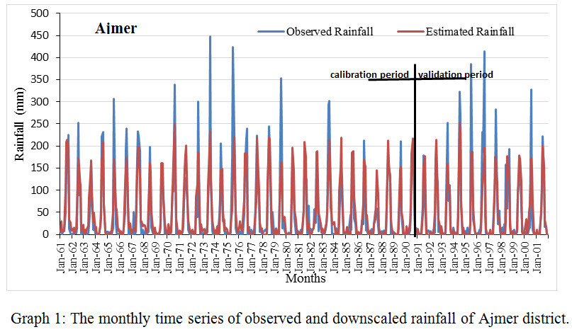Graph 1: The monthly time series of observed and downscaled rainfall of Ajmer district. Click here to view graph

 

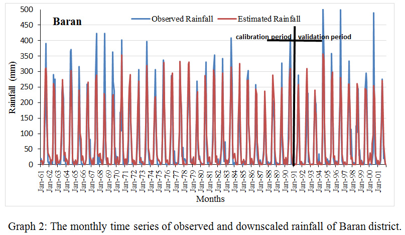Graph 2: The monthly time series of observed and downscaled rainfall of Baran district. Click here to view graph

 

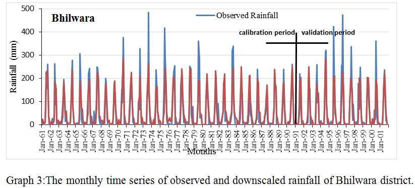Graph 3: The monthly time series of observed and downscaled rainfall of Bhilwara district. Click here to view graph

 

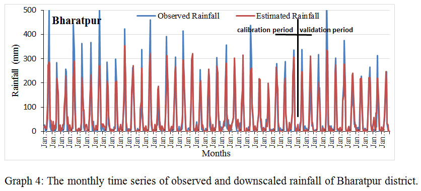Graph 4: The monthly time series of observed and downscaled rainfall of Bharatpur district. Click here to view graph

 

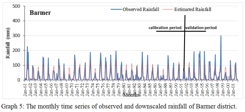Graph 5: The monthly time series of observed and downscaled rainfall of Barmer district. Click here to view graph

 

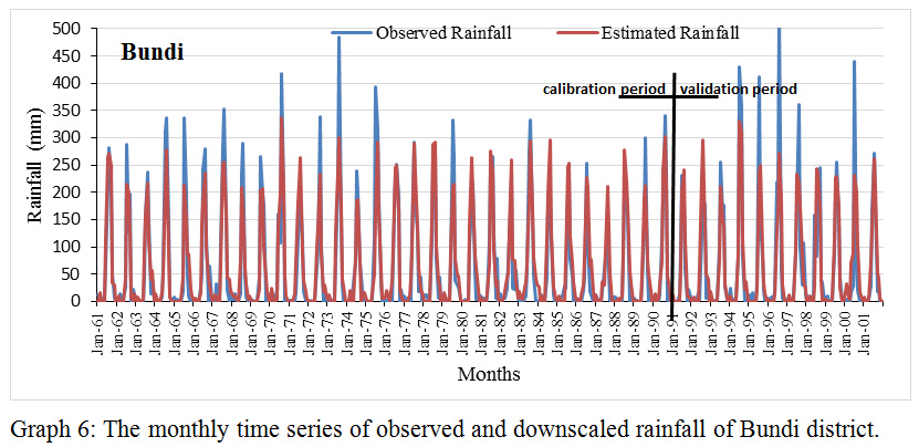Graph 6: The monthly time series of observed and downscaled rainfall of Bundi district. Click here to view graph

 

Graph 7: The monthly time series of observed and downscaled rainfall of Chittorgarh district. Click here to view graph

 

Graph 8: The monthly time series of observed and downscaled rainfall of Churu district. Click here to view graph

 

Graph 9: The monthly time series of observed and downscaled rainfall of Dausa district. Click here to view graph

 

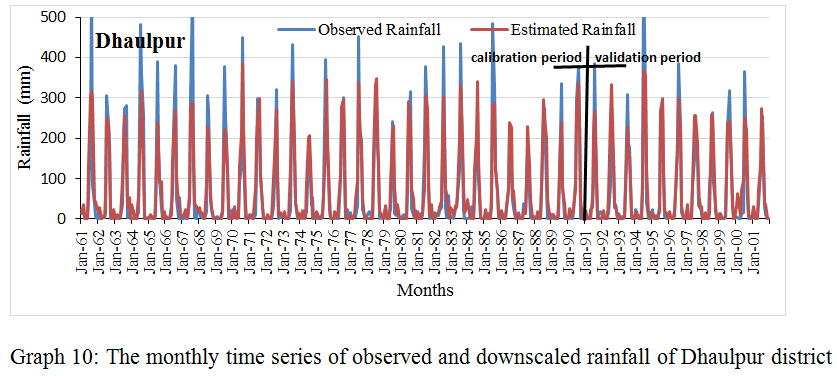Graph 10: The monthly time series of observed and downscaled rainfall of Dhaulpur district. Click here to view graph

 

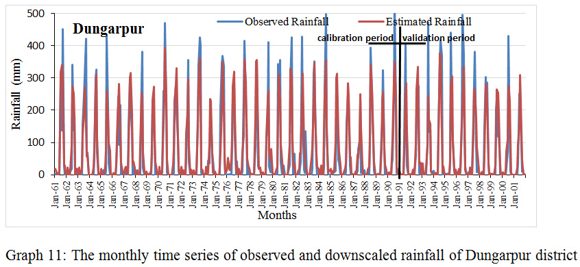Graph 11: The monthly time series of observed and downscaled rainfall of Dungarpur district. Click here to view graph

 

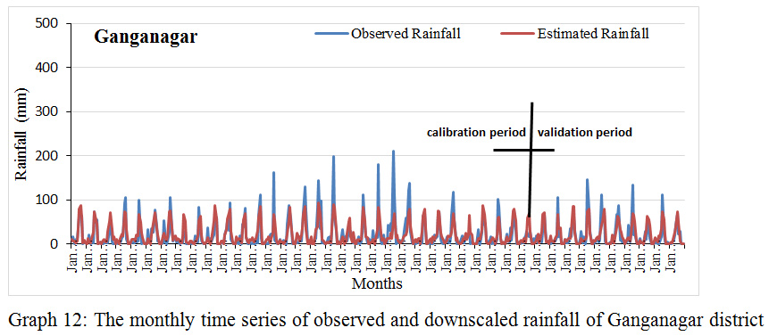Graph 12: The monthly time series of observed and downscaled rainfall of Ganganagar district. Click here to view graph

 

Graph 13: The monthly time series of observed and downscaled rainfall of Hanumangarh district. Click here to view graph

 

Graph 14: The monthly time series of observed and downscaled rainfall of Jaipur district. Click here to view graph

 

Graph 15: The monthly time series of observed and downscaled rainfall of Jaisalmer district. Click here to view graph

 

Graph 16: The monthly time series of observed and downscaled rainfall of Jalor district. Click here to view graph

 

 

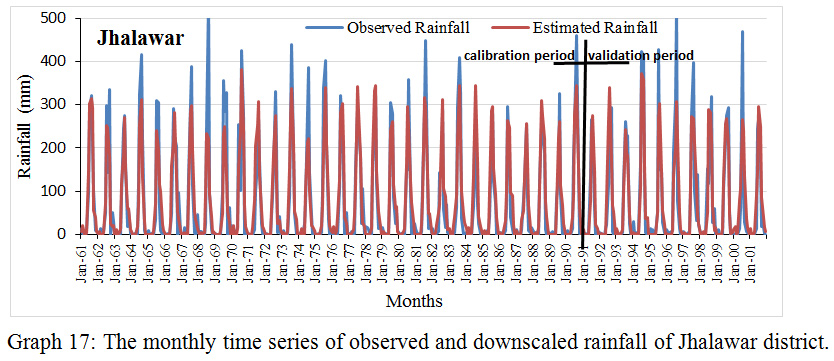Graph 17: The monthly time series of observed and downscaled rainfall of Jhalawar district. Click here to view graph

 

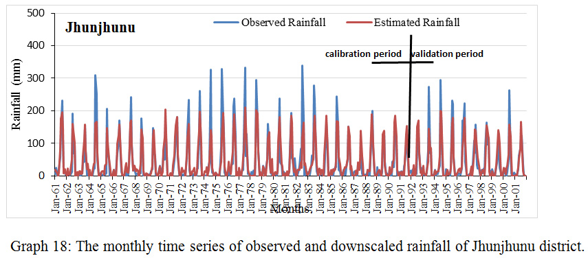Graph 18: The monthly time series of observed and downscaled rainfall of Jhunjhunu district. Click here to view graph

 

 

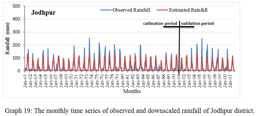Graph 19: The monthly time series of observed and downscaled rainfall of Jodhpur district. Click here to view graph

 

Graph 20: The monthly time series of observed and downscaled rainfall of Karauli district. Click here to view graph

 

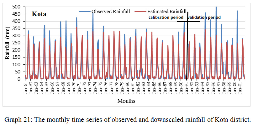Graph 21: The monthly time series of observed and downscaled rainfall of Kota district. Click here to view graph

 

Graph 22: The monthly time series of observed and downscaled rainfall of Pali district. Click here to view graph

 

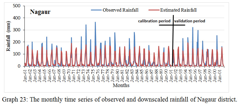Graph 23: The monthly time series of observed and downscaled rainfall of Nagaur district. Click here to view graph

 

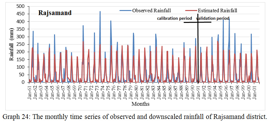Graph 24: The monthly time series of observed and downscaled rainfall of Rajsamand district. Click here to view graph

 

Graph 25: The monthly time series of observed and downscaled rainfall of Sikar district. Click here to view graph

 

Graph 26: The monthly time series of observed and downscaled rainfall of Sirohi district. Click here to view graph

 

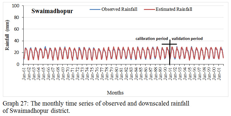Graph 27: The monthly time series of observed and downscaled rainfall of Swaimadhopur district. Click here to view graph

 

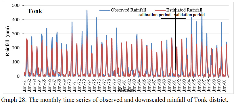Graph 28: The monthly time series of observed and downscaled rainfall of Tonk district. Click here to view graph

 

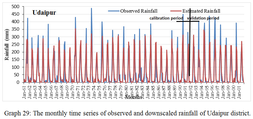Graph 29: The monthly time series of observed and downscaled rainfall of Udaipur district. Click here to view graph

 

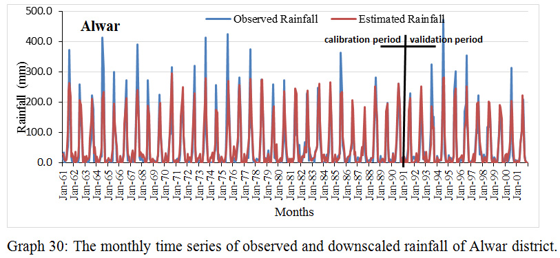Graph 30: The monthly time series of observed and downscaled rainfall of Alwar district. Click here to view graph

 

 

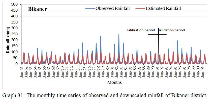Graph 31: The monthly time series of observed and downscaled rainfall of Bikaner district. Click here to view graph

 

 

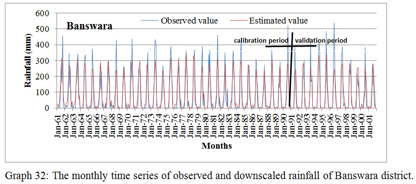Graph 32: The monthly time series of observed and downscaled rainfall of Banswara district. Click here to view graph

Appendix II: Box plot of all the districts of Rajasthan showing projected rainfall in MLR-A2 and B2 scenario.

A2 scenario   MLR-B2 scenario
 

Appendix II: a Click here to view appendix

 

Appendix II: b Click here to view appendix

 

Appendix II: c Click here to view appendix

 

Appendix II: d Click here to view appendix

 

Appendix II: e Click here to view appendix

 

Appendix II: f Click here to view appendix

 

Appendix II: g Click here to view appendix

 

Appendix II: h Click here to view appendix

 

Appendix II: i Click here to view appendix