A Review of Chronological Evolution of Air Quality Indexing Systems (1966 to 2021)
Dipsha Paresh Shah1,2
*
 and Dr. Piyushkumar Patel3
http://dx.doi.org/10.12944/CWE.16.3.5
Copy the following to cite this article:
Shah D. P, Patel P. A Review of Chronological Evolution of Air Quality Indexing Systems (1966 to 2021). Curr World Environ 2021;16(3). DOI:http://dx.doi.org/10.12944/CWE.16.3.5
Copy the following to cite this URL:
Shah D. P, Patel P. A Review of Chronological Evolution of Air Quality Indexing Systems (1966 to 2021). Curr World Environ 2021;16(3). Available From: https://bit.ly/3EZgzEz
Download article (pdf) Citation Manager Publish History

Introduction
The presence of harmful chemicals or compounds in the air such as particulate matters (PM10, and PM2.5), CO, O3, SO2, NO2, which not only lowers the quality of air but also deteriorates human health and overall quality of life is defined as air pollution. After industrialization, globalization and modernization have drastically changed the living standards with the introduction of gadgets like motorcycles, air conditioning systems which have made life simpler but also increased the pollution levels.
As per the estimation done by the World Health Organization (WHO), in developing countries, about 25% of all deaths may be due to environmental pollution. Due to increasing industrial development air pollution and its resultant adverse health impacts increases. A study by World Health Organization also revealed the possibility of risk of airborne diseases due to constant exposure to air pollution over a long time (WHO, 2009). Therefore, awareness of air pollution is necessary among citizens which leads to an increasing need for communication to the common public about the pollution levels. The simplest way to report the status of air quality to people is the AQI system. Around the world, various indexing systems have been established, but there is no universal indexing system, which can be used globally, in all conditions. The development of the indexing system starts in 1966 with considering only two pollutants; coefficient of haze (COH) and sulfur dioxide (SO2). The latest development in the air quality indexing system in the year 2021, six pollutants have been considered. This indexing system is based on the impact of contaminants on human health. Fuzzy set theories are very important to decide uncertain environmental conditions. Many researchers also developed the fuzzy modeling-based air quality indexing system, which is reviewed in a separate section in this paper. This present paper attempts to review these Air Quality Indexing Systems with its strength and limitations.
Review of Chronological Evolution of Air Quality Indexing Systems
The chronological evolution of air quality indexing systems since 1966is discussed in this section along with the number of pollutants considered, salient features of indexing systems, methods adopted for index formulation, and its limitations.
Green’s Index, 19661
Green’s Index is the first air Quality Index developed in 1966 by Marvin H. Green. This pollution index is based on only two parameters: i. Sulfur dioxide and ii. Smoke shade. The reasons for selecting these two parameters were that the quality index developer observed a strong correlation between these two parameters during New York’s air pollution episodes and also both the pollutants’ concentrations were observed very high during air pollution episodes. In this research, the hypothesis was that “there are certainly very high concentrations of sulfur dioxide in theair, which, when reacted with a similarly high concentration of particulate matters as represented as smoke shade measurements, can increase the death expectancy in the exposed population.”Three different categories concerning pollutants concentration are shown in table 1.
Table 1: Concentration Corresponding to Various Alert Levels.
|
Sulfur Dioxide |
Smoke Shade |
|
|
Desired Concentration |
≯0.06 ppm |
≯0.9 COH unit |
|
This standard was set by soviet scientists based on the daily average level of the USSR. |
This number was selected as many control agencies considered the 0.9 COH as light, and this was the monthly average measured in summer in Philadelphia. |
|
|
Alert Concentration |
0.3 ppm |
3 COH unit |
|
This condition is a sign of unpleasant conditions in the atmosphere, taking into consideration the recommendation of Dr. Collings that 0.3 ppm sulfur dioxide along with the smoke shade of 4 COH is considered as the level of alert. |
This number was selected because the smoke shade range is labelled very heavy after 3 COH units |
|
|
Extreme Concentration |
1.5 ppm |
10 COH unit |
|
It is the most unusual scenario for sulfur dioxide to reach or exceed 1. 5ppm. |
It is the most unusual scenario and it is rarely attained therefore it is considered the most dangerous case. |
The author developed the equations to convert the pollutants’ concentration to index value based on power function. The conversion from pollutant level to the index number is done by the power function represented as Eq. 1 and Eq. 2.
I = 84.0*S0.431 ……………………….Eq. 1
I = 26.6*C0.576 …………………………Eq. 2
Where, S = concentration of sulfur dioxide, ppm
C = smoke shade level in COH per 1000 feet.
To qualify the air based on two pollutants combined index was formed using equation 3.
Combined Index = 0.5* (Sulfur dioxide Index + Smoke Shade Index)…………………Eq. 3
This index is only relevant and applicable in winter (colder season). Based on the above-mentioned equations,3 Alerts must be issued. The first alert, second alert, and third alert were issued by the control agency’s chief administrator at an index value of 50, 60, and 68 respectively. Limitations of this index are that it includes only two pollutants; SO2 and COH. It is ambiguous and eclipsing in nature. This indexing system was for activating regulating actions during air pollution episodes rather than air quality data reporting to the people. The index level along with the description is tabulated in table 2.
Table 2: Desired Levels Along with Descriptors.
|
Index |
SO2(ppm) |
COH |
Descriptors |
Remarks |
|
0-25 |
0.06 |
0.9 |
Desired |
Clean, Safe Air |
|
25-50 |
0.3 |
3 |
Alert |
Potentially Hazardous |
|
50-100 |
1.5 |
10 |
Extreme |
Curtail Air Pollution Sources |
Most Undesirable Respirable Contaminants Index (MURCI),19682
In Detroit, this index is used to inform daily the status of the quality of ambient air to the people. It was transmitted by local radio stations, at 8:30 a.m. daily. Only one pollutant was considered in the development of the index; i.e.coefficient of Haze (COH), as shown in Eq. 4.
MURC = 70*X0.7 ……………… Eq.4
Where,
X = COH units
Equation 4 was derived so that if the COH value was between 0.3 to 2.15, MURC index values were between 30 to 120. The breakpoint concentration for the MURC index is tabulated in table – 3. The limitation of the index is that there is no correlation with SPM if the index values are more than 120.
Table 3: Breakpoint Concentration for MURCI.
|
Index |
COH |
Descriptors |
|
0-30 |
0.3 |
Extremely Ligt Contamination |
|
31-60 |
0.92 |
Light Contamination |
|
61-90 |
1.53 |
Medium Contamination |
|
91-120 |
2.15 |
Heavy Contamination |
|
>120 |
>2.15 |
Extremely Heavy Contamination |
Fen Stock Air Quality Index (AQI), 19692,3
In 1969, Fenstocket. al. developed the “Fenstock Air Quality Index” to evaluate the comparative air pollution severity, and relate it to 29 United States cities. This was the first index, in which meteorological conditions of each city and source emissions data were used to estimate air pollutant concentrations. The equation formed for Fenstock AQI is shown as Eq. 5.
AQI = WI * iI ………………..Eq. 5
Where,
Wi = TSPM, SO2, and CO weightages
Ii = TSPM, SO2, and CO sub-index
The limitation of the index is that it is applied to only a square city area with the wind direction parallel to one side. The indexing system was based on the assumption of neutral stability conditions of ambient air with the continuous source distribution. It cannot be used for daily air quality reports. It can be used for the estimation of total air pollution probability in a city.
Air Pollution Index, Ontario (API), 19704
API was developed by Shenfeld et. al. in 1970 for Ontario city. The purpose to design the index was to update the people about the pollution levels and to compare the present pollutants’ concentration with the concentration of pollutants during "Air Pollution Episodes”. The index was designed as shown in Eq. 6 based on continuous monitoring of SPM and SO2. The SPM concentrations were determined as soiling index in units of coefficients of haze per 1000 feet of air. Air Pollution Index (API),
API=0.2*(30.5 COH + 126.0SO2)1.35 ………….Eq. 6
Where,
COH =24 hrs. the average concentration of coefficient of the haze (Running average)
SO2 = Concentration of SO2 of 24 hrs. (Running average), ppm
The API range was from 0 to 100. API range with relevant description is tabulated in table 4.
Table 4: API Range and Description Curtail.
|
API Range |
Description |
|
0 – 32 |
Acceptable, at these levels concentration of SPM and SO2 have an insignificant effect on human health. |
|
33 – 50 |
Advisory, the first alert is issued. An order may be issued by the minister to major source contributors to curtail their activities. |
|
51 – 75 |
Issue of the second alert. The minister may mandate sources for further restriction in operations. |
|
76 – 100 |
The threshold level for air pollution episode, restrictions of all sources not important for the health of people, or safety may be required. |
|
>101 |
Air Pollution Episode may occur if measures have not been taken. |
Oak Ridge Air Quality Index (ORAQI), 19715
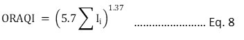
This indexing system is developed in the National Laboratory of Oak Ridge in 1971. Five contaminants; particulate matter, photochemical oxidants, CO, SO2, and NO2 had been selected for the index calculation. The index’s aggregation function is non-linear as represented as Eq. 7 and Eq. 8. The index is subjected to eclipsing and ambiguity is the limitation of the index.
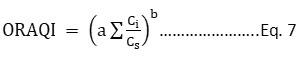
Ii= (C/Cs)i
C =Contaminant concentration
Cs = Contaminant Standard
Ii = sub-indices of Pollutants; SPM, CO, SO2, NO2, and Photochemical Oxidants
Table 5: Pollutants’ Standard Concentrations for Index.
|
Pollutant |
Standard Value (24 Hours average) |
|
Photochemical oxidants |
0.03 ppm |
|
Sulfur dioxide |
0.10 ppm |
|
Nitrogen dioxide |
0.2 ppm |
|
Carbon monoxide |
7 ppm |
|
Particulate matter |
150 µg/m3 |
U. S. EPA Pollutant Standards Index (PSI), 19766
In August 1976, the US EPA evolved the pollutant standards index (PSI). The linear interpolation method was used in the development of the index, in which the concentrations of air pollutants were converted to a standard number, known as a sub-index. The maximum sub-index value of pollutants was reported as the overall index of air quality. The index is a maximum operating function base, represented as Eq. 9. PSI included five pollutants: TSPM, O3, NO2, SO2, and CO. If pollutant concentration and sub-index value for a given pollutant are represented as x and y respectively, a segmented linear function is represented asEq.10. The breakpoint concentration of pollutants is shown in table 6.
PSI = max (y1, y2 … y6)………………….Eq. 9
For ai < x ≤ ai+1,
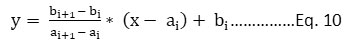
Where, i = 1, 2…6
bi = Index Value
ai = Pollutants breakpoint concentration
x = Pollutants measured concentration
Table 6: Breakpoint Concentration of Pollutants for PSI.
|
Sr. No. |
Index |
Total Suspended Particulate Matters (TSPM), μg/m3 |
Ozone (O3), |
Carbon Monoxide (CO), mg/m3 |
Nitrogen Dioxide (NO2), μg/m3 |
Sulfur Dioxide (SO2), |
|
1 |
0 |
0 |
0 |
0 |
* |
0 |
|
2 |
50 |
75 |
80 |
5 |
* |
80 |
|
3 |
100 |
260 |
160 |
10 |
* |
365 |
|
4 |
200 |
375 |
400 |
17 |
1130 |
800 |
|
5 |
300 |
625 |
800 |
34 |
2260 |
1600 |
|
6 |
400 |
875 |
1000 |
46 |
3000 |
2100 |
|
7 |
500 |
1000 |
1200 |
56.7 |
3750 |
2620 |
*No standards or episode criteria exist at these levels. So, the sub-index can not be calculated.
The major limitation of this index is that the index values are only on the basis of the concentration of one pollutant at a time. The index can’t show whether concurrently, two or more pollutants exceed the standards or not. It is free from ambiguity and eclipsing. However, it does not account for the other harmful contaminants to human health.
Integral Air Pollution Index (IAPI), 19937, 8
It is constructed on the basis of pollutants’ maximum permissible concentration (MPC)which was suggested by Bezuglayaet al. (1993). It allows a complex estimation of air pollution in urban areas. To compare air pollution levels in various cities, the same number of pollutants were considered during the calculation of IAPI. It was developed for Russian cities and based on the measurement of the concentration of phenol, Benz(a)pyrene (BP), Formaldehyde, and Metals. Maximum permissible concentration (MPC) is a concentration of pollutants, which directly or indirectly does not affect human health and prosperity. Also, the pollutant’s concentration at which people do not feel less efficient, and does not deteriorate sanitary conditions. The index is the ratio of pollutant concentration to the maximum permissible concentration as represented in Eq. 11.
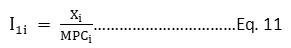
Where, xi = Concentration of ith pollutant
I1i = Air pollution index (Sub-index) of the ith pollutant
MPCi = ith pollutant’s maximum permissible concentration
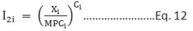
In the development of the IAPI, the assumption was taken that on human health, the effect of individual pollutants at the maximum permissible concentration (MPC) is equal, but with an increase of their concentrations beyond maximum permissible level, the degree of hazard rises differently for different pollutants. Pollutants are categorized into four classes of hazards by the health experts. The first category is classified as the most hazardous class which includes Benz(a)pyrene, Lead, Mercury, and Nickel. The second category includes copper oxide, nitrogen dioxide, formaldehyde, and phenol. The third category includes suspended particulate matter and sulfur dioxide and the fourth category includes carbon monoxide. The values ofCi for the four hazardous class is tabulated in table 7. Air pollution index (API) along with degree exponent is represented as Eq. 12.
The integral air pollution index (IAPI) was estimated by arithmetic summation of sub-indexes, represented as Eq. 13.
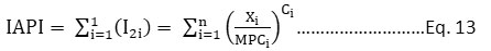
Table 7: The Average Values of Ci for Four different Danger Classes.
|
Danger Class |
Cj |
|
1 |
1.7 |
|
2 |
1.3 |
|
3 |
1 |
|
4 |
0.9 |
The limitation of this index is that by nature, it is ambiguous, which may lead to false alarms when calculated to be hazardous. To eliminate this limitation, Swamee and Tyagi (1999) developed a quantitative tool-based air pollution index through which air pollution status can be conveyed consistently. They introduced ambiguity and eclipsing free aggregating function for the air pollutants sub-indices as shown in Eq. 14. After extensive study, an exponent value p = 0.4 was derived and given in the aggregation function to eliminate the ambiguity.
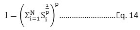
p = an exponent
Si = ith pollutant’s sub-index
N= Number of sub-indices
I = Aggregate index
A Simple Air Quality Index, 19939
The index was designed for Helsinki, the capital of Finland in 1993 to update the people especially a layman about present air quality status in an understood way. The pollutants considered in the AQI wereCO, NO2, SO2, O3, and PM10. The index was based on the impact on human health and the long-term impact on flora, fauna, and materials. Hourly sub-indexes were calculated for all considered pollutants through segmented linear function and the highest value sub-index becomes the AQI for that hour i.e. the maximum operating function-based index. Moving averages are considered for 24 hours and 8 hours average concentration. The index range was from 10 to 150. The breakpoint concentration of pollutants and pollutants standards is tabulated in table 8. Index categories along with index color and description are tabulated in table 9. The limitation of the index is that the collective effects of air pollutants are not considered due to the lack of enough scientific evidence.
Table 8: AQI Values with Breakpoint Concentration of Pollutants.
|
Pollutants |
Carbon "Monoxide (CO), mg/m3 |
Nitrogen Dioxide |
Sulfur Dioxide |
Ozone (03), |
Respirable Suspended Particulate Matter |
|||
|
|
1hr. |
8 hr. |
1hr. |
24 hr. |
1hr. |
24 hr. |
1hr. |
24 hr. |
|
Standards |
20 |
8 |
150 |
70 |
250 |
80 |
150* |
70 |
|
Index Values |
|
|||||||
|
10 |
0.5 |
0.5 |
7 |
7 |
4 |
4 |
50 |
IO |
|
50 |
4 |
4 |
35 |
35 |
40 |
40 |
75 |
35 |
|
100 |
20 |
8 |
150 |
70 |
250 |
80 |
150 |
70 |
|
150 |
30 |
12 |
225 |
105 |
375 |
120 |
225 |
105 |
*as per WHO Guidelines (1987)
Table 9: AQI Categories.
|
Index |
Color |
Description |
|
< 50 |
Green |
Good air quality, no health effect, a slight effect on the ecosystem. |
|
51 – 100 |
Yellow |
Fair air quality, adverse effect unlikely, the effect on nature and material. |
|
101 – 150 |
Orange |
Safe air quality, the possibility of adversarial effects on sensitive people, noticeable effects on materials and vegetation. |
|
>150 |
Red |
Possibility of adversarial effects on sensitive people. Marked effect on flora, fauna, and materials. |
U. S. EPA Air Quality Index, 199910
The AQI was revised by U.S. EPAin 1999. The agency changed the name from Pollutant Standards Index (PSI) to Air Quality Index (AQI). It is a tool used to report air quality status to the public in a simple manner, as the index is uniform and easy of understanding. The index incorporates six criteria pollutants: PM10, PM2.5, O3, SO2, CO, and NO2. The index is divided into six different categories. If the index value is more than 100, the US EPA agency starts to update the pollutant-specific sensitive group, with specific colors. The agency also included 8-hour average O3 concentrations scaling range for the ozone (O3) sub-indices. It also included a new sub-index of PM2.5. During the revision, the agency also modified the breakpoint values of the sub-indices for PM10, SO2, and CO. The index range was from 0 to 500, but the index range 101 to 200 has also been split as 101 to 150 and 151 to 200. The revised category of the index value, descriptors, and colors are shown in table 10. The breakpoints for the pollutants sub-indices are tabulated in table 11. The main objective of modifications in the US EPA index was to reinforce the index system’s health implication, particularly for the population sensitive to poor air quality. World widely, this system has been adopted due to its simplicity and accuracy.
Table 10: US EPA Index Values, Descriptors and Specific Colors.
|
Sr. No. |
Index Values |
Descriptor |
Color |
|
1. |
0-50 |
Good |
Green |
|
2. |
51-100 |
Moderate |
Yellow |
|
3. |
101-150 |
Unhealthy for sensitive group |
Orange |
|
4. |
151-200 |
Unhealthy |
Red |
|
5. |
201-300 |
Very Unhealthy |
Purple |
|
6. |
301-500 |
Hazardous |
Maroon |
Table 11: Breakpoints for Pollutants Sub-Indices.
|
AQI Value |
O3, ppm |
PM2.5, μg/m3 |
PM10, μg/m3 |
CO, ppm |
SO2, ppm |
|
|
|
8hr. |
1hr. |
24hr. |
24hr. |
8hr. |
24hr. |
|
50 |
0.07 |
- |
15 |
50 |
4 |
0.03 |
|
100 |
0.08 |
0.12 |
65 |
150 |
9 |
0.14 |
|
150 |
0.1 |
0.16 |
100 |
250 |
12 |
0.22 |
|
200 |
0.12 |
0.20 |
150 |
350 |
15 |
0.30 |
|
300 |
- |
0.40 |
250 |
420 |
30 |
0.60 |
|
400 |
- |
0.50 |
350 |
500 |
40 |
0.80 |
|
500 |
- |
0.60 |
500 |
600 |
50 |
1 |
Aggregate Index, 199911
If the index is based on linear sum and root sum square form, it suffers from ambiguity. To omit the ambiguity of the Integral Air pollution Index (IAPI), this index was developed. While the maximum operating function-based index does not consider the change in the remaining pollutants. Therefore, Swamee and Tyagi developed an aggregate index in 1999, which was free from ambiguity and eclipsing. In the formation of the index, the index developers considered five pollutants; TSPM, SO2, CO, NO2,andO3. The developed aggregation index is represented as Eq. 15. It was concluded that for an exponent value P = 0.4, the aggregation index included the value of all the sub-indices, and ambiguity was minimized. The aggregation index can be used to report air pollution data uniformly.
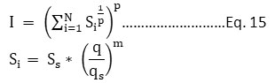
Where,
I = Aggregate Index
Si = ith pollutant’s sub-index
Ss = Scaling coefficient, 500 in NAAQS and 1 in Russian air pollution monitoring studies
m and p = an exponent
q = pollutant concentration
qs = Standard concentration of pollutant
Revised Air Quality Index, 200412
This index was developed by joining Shannon’s entropy function and pollutant standard index (PSI). It is a contextual mean entropy and arithmetic index. Combining entropy function rectifies the deficiency of PSI that it identified only one pollutant level at a time, hence it was difficult to ascertain that whether more than one pollutant exceeds standards or not. Therefore, this index with comparative index function was developed which allows more diffusion and makes it simpler to find the biggest index value. The formula developed as RAQI is represented as Eq. 16.
RAQI =

In the RAQI, five pollutants had been considered and compared: PM10, SO2, NO2, O3, and CO. In the equation, the first factor represents the maximum value of each sub-index, i.e. maximum operating function is used in the first factor. The maximum operating function has been considered in the equation to reduce the eclipsing irregularity. In the second factor, the numerator is the summation of the daily arithmetic mean of each sub-index, while the denominator is the yearly mean multiplied by the summation of the daily mean. The third factor is the background arithmetic average entropy index value. Log 10 of the entropy function is defined as the maximum operating function of I1...In. The entropy function is a modifier that helped to stop mathematical deviation to extremely large values. As compared with PSI, the RAQI value is always greater than the PSI value. RAQI poorly predicts the short-term health impact or short-term air quality. This index is more useful to predict long-term health impacts and long-term air quality.
Pollution Index (PI), 200413
Two different pollution indexes had been established and implemented in Naples city (Italy). For the development of the index, data was collected and analyzed from nine monitoring stations in 2003. One background station, two stations in residential areas, four stations in high traffic regions, and two stations that monitored photochemical pollution were among the nine monitoring stations. The aim of the development of the pollution index (PI) was to evaluate the air pollution status with its consequence on the health of human beings. The pollution index is a modified version of US EPA AQI, considering the standards governing in Europe. The pollution index (PI) was re-evaluated considering the aggregation of air pollutants.
The pollution index range is from 0 to 100, divided into five different categories instead of six categories of the US EPA AQI. The breakpoint concentration of different pollutants along with pollution category, pollution index range, and pollution categories definition is shown in table 12. The pollution index was determined by linear interpolation among the cutoff values shown in table 12. The first two levels index range were recognized by EC directives, while the 3rd and 4th index range was established through the epidemiology of pollutants. To communicate the air quality to the population, clouds were used as symbols corresponding to pollution categories. The formula to calculate the pollution index of ith pollutant on the jth station is represented as eq. 17. The highest value of the pollutant’s sub-index was represented as the pollution index of that site as shown in eq. 18.
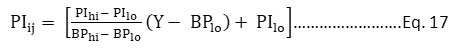
Where, Y = the daily reference concentration
BPhi = The lowest reference concentration that is more than or equal to Y
BPlo = The highest reference concentration that is more than or equal to Y
PIhi = The PI value corresponding to BPhi
PIlo = The PI value corresponding to BPlo
PIj = maxâ¡(PIij ) ………………………………………………….Eq. 18
Table 12: The Pollution Index with a Breakpoint of Sub-Indices.
|
Pollution Index |
Pollution Category |
Pollution Category Definition based on pollution concentration |
Pollution Category Symbol |
PM10, 24 hrs., μg/m3 |
NO2, 1 hr, μg/m3 |
CO, 8h, mg/m3 |
SO2, 24 h, μg/m3 |
O3, μg/m3 |
|
|
1 h |
8 h |
||||||||
|
25 |
Good Quality |
Below are the standards established by EC, assuming that no impact on the environment and health of people. |
|
20 |
40 |
4 |
20 |
- |
65 |
|
50 |
Low Pollution |
Below are the standards established by ECf for the protection of the health of people. |
|
50 |
200 |
10 |
125 |
180 |
120 |
|
70 |
Moderate Pollution |
Above the standards established by EC |
|
144 |
400 |
11.6 |
250 |
240 |
180 |
|
85 |
Unhealthy for sensitive groups |
Affect the sensitive groups (Children, Asthmatics...) |
238 |
950 |
15.5 |
500 |
324 |
223 |
|
|
100 |
Unhealthy |
Affect all populations, higher effect on sensitive groups |
|
500 |
1900 |
30 |
1000 |
600 |
500 |
The pollution index has been developed for single pollutants. In a mixture, pollutants may have synergetic or additive effects on human health. Synergistic effects of pollutants have not been developed yet. In the pollution index determination procedure, other pollutants do not contribute to the estimation of the index. The pollution index value may be higher than that obtained by the maximum operating function and would represent the actual situation if synergistic effects would be considered. To consider the synergistic effects of pollutants, Murena tried to modify the pollution index as shown in Eq. 19, based on the procedure applied in industrial hygiene for validating threshold values in the scenario of air pollutants’ mixture.
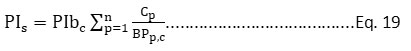
Where,
PIs = Pollution index of a particular site
Cp = Concentration of pollutant (P)
BPp,c = For pollutant P, the lower range of scale, corresponding to each category (C), as shown in Table 12.
PIbc = the lowest value of PI relating to maximum pollution category C
With this assumption, Naples’ air quality data had been re-described and pollution index (PIs) is re-calculated. There is a significant difference between the results generated due to the maximum operating function-based pollution index and the synergetic effect of the pollutants-based pollution index. The results showed that the additive effects of pollutants strongly influenced the air quality evaluation. If air pollutants are in the same category, additive effects can be expected and have the same effects on the health of human beings. This is relevant to all five pollutants considered in the modified pollution index. So, the result obtained through a modified pollution index was overestimated than the actual pollution index.
Air Quality Depreciation Index (AQDI), 200614
An index was formed that measures ambient air quality deterioration ranging between 0 and - 10. The index was applied on monitoring data of ten different monitoring stations of coal mining areas of Kobra Industrial belt(approx. 530 square km coverage) for one year. AQDI measures air quality deterioration considering the amalgamation of factors that affect human health, aesthetic, and biophysical attributes on an absolute scale of environmental quality, which is not dependent on NAAQS. The value function graphs, which are based on long-term health impacts, are used in the development of AQDI. A value of index; 0 denotes the most desired air quality i.e. no decline in air quality. While a value of index-10 represented the worst air quality or maximum deterioration. The index is formulated as shown in Eq. 20.

Where,
AQi=ith parameter’s air quality
CWi = ith parameter’s composite weight
n = Number of selected pollutants
The AQi values were found from the value function graph, ranging from 0 to 1; for corresponding pollutant concentration, 0 signifies poorest air quality and 1 signifies the good air quality. The value of CWi was computed using Eq. 21.
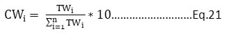
Where,
TWi =ith parameter’s total weight
= HWi+AWi+BPIWi
Where,
HWi= ith parameter’s weight of human’s health
AWi= ith parameter’s aesthetical weight
BPIWi = ith parameter’s biophysical impact weight
In TWi computation, a weight ranging from 1 to 5 was assigned subjectively to HWi, AWi, and BPIWi by a team of experts. One was assigned to the least important factor and five was assigned to the most important factor. The calculation of the composite weight of different pollutants and assigned values are represented in Table 13. This index represents even small changes in air quality in a more simple and meaningful way and like AQI it doesn’t simply make comparisons to NAAQS to assess air quality.
Table 13: Assigned Values and Composite Weight of Pollutants.
|
Pollutants |
HWi |
AWi |
BPIWi |
TWi |
CWi |
|
SPM |
3 |
4 |
4 |
11 |
3.1 |
|
SO2 |
4 |
1 |
4 |
9 |
2.5 |
|
NOx |
3 |
2 |
3 |
8 |
2.2 |
|
TSP X SO2 |
5 |
1 |
2 |
8 |
2.2 |
The index can be used to prepare a periodic air quality deterioration map representing the possibility of environmental damages. The AQDI is not geographically specific and can be used for the number of pollutants. The index can also be used for various applications and situations.
An Aggregate Air Quality Index, 200715
George Kyrkiliset. al. developed an index considering aggregate effects of pollutants and European standards for Athens city, the capital of Greece. In Athens, there were serious air pollution problems. They considered five criteria pollutants: PM10, CO, O3, SO2, and NO2. Two different models were adopted to develop AQI for the Athens area; one was the maximum air quality index (AQI) model and the second was an aggregate air quality index (AQI) model. In Athens, four stations were selected and all five pollutants were monitored. In the first model, the maximum operating function-based air quality index was calculated for each station. Then the median of maximum operating function based air quality index of four stations is considered to be the entire city’s AQI. Due to the limited availability of data, the index creator imposed the constraint that, for a given station, the maximum operating function-based AQI value must be based on a minimum of three pollutants, two of which must be PM10 and NO2. These two pollutants were selected, as both pollutants were needed in the aggregate index calculation. For the city’s atmosphere, PM10is considered severe problematic and NO2 concentration was very high in the city and also it acts as an ozone precursor.
The available data of air pollutants from 1983 to 1999 of all four selected monitoring stations were analyzed for the proposed index development. For each day, the maximum AQI value (Imax) and aggregate AQI value (Iag) of the city were calculated. The comparison was done between two indexing systems; an aggregate AQI with USEPA-based maximum AQI model adjusted for European conditions. To get the USEPA-based AQI based on European conditions, European Union standards, which are more stringent replaced the Clean Air Act (CAA) standards. The pollutants breakpoint concentration range for all air quality categories is shown in table - 14.
Table 14: A Modified Breakpoint Values according to European Standards for Calculating USEPA based AQI.
|
Air Pollution Category |
AQI |
CO |
NO2 |
O3 |
O3 |
PM10 |
SO2 |
|
Good |
0 – 50 |
0 – 4.7 |
0 – 152 |
0 – 137 |
0 – 91 |
0-18 |
0 - 30 |
|
Moderate |
51 – 100 |
4.7 – 10 |
152 – 200 |
137 – 180 |
91 – 120 |
18 – 75 |
30 – 125 |
|
Unhealthy for sensitive groups |
101 – 150 |
10 – 13 |
200 – 262 |
180 -236 |
120 – 149 |
75 – 124 |
125-194 |
|
Unhealthy |
151 – 200 |
13 – 16 |
262 – 326 |
236 – 294 |
149- 177 |
124 – 172 |
194 – 264 |
|
Very unhealthy |
201 – 300 |
16 – 32 |
326 – 646 |
294 – 582 |
177- 534 |
172 – 206 |
264 – 524 |
|
Hazardous |
301 – 400 |
32 – 43 |
646 – 806 |
582 – 726 |
534-667 |
206 – 245 |
524 - 698 |
|
Severe |
401 - 500 |
43 – 54 |
806 - 966 |
726 - 870 |
667-799 |
245 - 294 |
698 - 872 |
In the second model, the aggregate air quality index was calculated for four stations. The whole city's AQI was calculated by selecting the median of the four AQIs.In the aggregate model, the sub-index was calculated based on each pollutant’s concentration. It is the quotient of pollutant concentration (q) to its standard value (qs) as represented in Eq. 22.
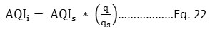
AQIi = ith pollutant’s sub-index
AQIs = Scaling coefficient equal to 500
The most appropriate aggregate function, considering the combined effects of all pollutants was developed by Swamee and Tyagi in 1999.
So, G.Kyrkiliset.al.adopted the same function represented as Eq. 23 to compute an aggregate AQI for Athens.
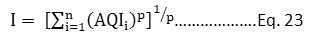
Where,
I = the aggregate air quality index/an overall AQI
P = Constant, 2.5 had been adopted for this study
The comparison of aggregate value model and maximum value model for the Athens city observed that about 60% of days; aggregate AQI value was in unhealthy conditions, while about 35% of days; the maximum AQI value was in unhealthy conditions. The comparison revealed that the aggregate index evaluated contaminants' vulnerability to the population more effectively than the maximum operating function-based US EPA index because aggregate AQI considered the influence of all monitored pollutants. The aggregate model is more effective to report to the people to keep them healthy in a city. It can apply as a managerial tool to prepare mitigation policies and to implement active actions.
CITEAIR’s Common Air Quality Index (CAQI), 200716
This index was developed as a part of the CITEAIRprojectinEurope for website development, presenting a comparison of European cities’ air quality. In 2006, the CITEAIR project was launched, with contributions from the five main cities. For the development of CAQI, two types of locations were considered: i. Roadside monitoring locations, and ii. Locations represent average city background conditions. The CITEAIR aimed to provide a unique index and mark a difference between city background stations and traffic stations. The CAQI is estimated by the linear interpolating method, according to the breakpoint values given in table 15. The final index is the maximum value of the sub-indices of each pollutant. The traffic index contains PM10, and NO2 with CO considered as a supplementary element. The city background index contains PM10, O3, and NO2 with SO2 and CO as supplementary elements. In the majority of the cities, the supplementary elements would hardly ever decide the index but in urban areas having industrial pollution or seaport, SO2 may occasionally be responsible for the index. The CAQI range is from 0 to 100. This indexing system can be used to compare real-time city air quality. It can be used either for daily or hourly indexes. Due to the non-availability of forecasting facilities in every city, an hourly index is considered. Hourly index proves to be dynamic because it ensures frequent visits to a website. The European directives declare daily averages and many cities of Europe do not even report hourly indexes. Due to the above-mentioned reasons, for RSPM averaging time increase from one hour to twenty-four hours. As the averaging time increases, the concentration value of particulate matter decrease. Hence in table 15, for PM10, breakpoint concentration value for averaging time of 1 hr and 24 hrs. were given. The limitation of CAQI is that the index does not consider the adverse impact due to the synchronicity of all the pollutants, pollutant aggregation, spatial aggregation, and uncertainty measures and health.
Table 15: Breakpoint Values of Pollutants for the CAQI.
|
Index class |
Index Value |
Traffic |
|
Citv back 2 round |
||||||||
|
Mandatory Pollutant |
Auxiliary pollutant |
|
: Mandatory pollutant |
Auxiliary pollutant |
||||||||
|
NO: |
PM10 |
co |
|
NOi |
PM 10 |
03 |
co |
SOz |
||||
|
I .hr |
I .h.r |
24 .hr |
S.hr |
|
I hr |
I h.r |
24 hr |
I .hr |
S h.r |
I 1.t.r |
||
|
Very low |
0 |
0 |
0 |
0 |
0 |
|
0 |
0 |
0 |
0 |
0 |
0 |
|
25 |
50 |
25 |
12 |
5000 |
|
50 |
25 |
12 |
60 |
5000 |
50 |
|
|
Low |
26 |
51 |
26 |
13 |
5001 |
|
51 |
26 |
13 |
61 |
5001 |
51 |
|
50 |
100 |
50 |
25 |
7500 |
|
100 |
50 |
25 |
120 |
7500 |
100 |
|
|
Mediwn |
51 |
101 |
51 |
26 |
7501 |
|
101 |
51 |
26 |
121 |
7501 |
101 |
|
75 |
200 |
90 |
50 |
10,000 |
|
200 |
90 |
50 |
180 |
10,000 |
300 |
|
|
High |
76 |
201 |
91 |
51 |
10,001 |
|
201 |
91 |
51 |
181 |
10,001 |
30·1 |
|
100 |
400 |
180 |
100 |
20,000 |
|
400 |
180 |
100 |
240 |
20,000 |
500 |
|
|
Very high ' |
>100 |
::>400 |
>180 |
>100 |
>20,000 |
|
>400 |
>180 |
>100 |
>240 |
>20,000 |
>500 |
New Air Quality Index (NAQI), 200917
The USEPA AQI gives a general assessment of the quality of air; without considering the synergetic effects of air pollutants. So, to overcome this limitation, the authors calculated the factor analysis aided by principal component analysis (PCA) based new air quality index (NAQI). In the development of the NAQI, the deficiencies of the US EPA method tried to be incorporated. The criteria pollutants: PM10, CO, and SO2 had been considered for determining NAQI and US EPA AQI for Delhi. In November, three additional parameters were monitored: NO2, O3, and NO. Total ten sites were selected as a sampling site covering the whole area of Delhi, out of ten sites; four sites were situated on the inner ring road, another four sites were situated on the outer ring road and the remaining two sites were situated on JNU Campus, situated in South Delhi. The 2003 – 04 years were divided into four seasons: monsoon (July - September), post-monsoon (October - November), winter (December - March), and summer (April - June). A total of eighteen representative days per season were selected for the study. The measurements for air pollutants were carried out continuously for 24 hours for the two sites of JNU. While the remaining eight sites, measurements were done for a period of four hours each in the evening and the next day morning for four hours for the same site. Automatic electronic monitors are installed in the mobile air pollution laboratory to monitor the air pollutants.
Seasonal effect on NAQI values
Winter Season
In winter, the highest index values were observed due to prevailing climatological conditions in north India and due to less dispersion of pollutants. High pressure in winter, in this region, is responsible for atmospheric stability, which results in more stagnant air masses and less circulation of air.
Summer and Monsoon Season
In summer, index values were observed high due to extreme dust storms covering Delhi’s atmosphere. During monsoon, comparatively, the value of NAQI is very small due to changes in wind direction, wash out of air pollutants due to precipitation, and dispersion of air pollutants due to high wind velocities.
Post-Monsoon Season
Air quality is comparatively better than summer and winter with exception of October which is mainly due to lighting crackers due to festivals of Diwali and Dussehra.
PCA
Principal Component Analysis (PCA) is a widely used factor analysis method. The main aim of PCA is to consider the total deviation amongst the 'n' number of variables (subjects) in p- dimensional space by creating a new set of orthogonal and uncorrelated composite variates. Consecutive composite random variables will consider a small portion of the whole deviation to generate linear combinations. The first principal factor (composite) will have the largest alteration; the second principal component will have alteration larger than the third but smaller than the first, and so on. To develop the composite (overall) AQI, if the first few composites (principal components) have more than 60% of the total variance, then there are no requirements for taking more principal components (PCs). The principal components method can be applied by using the original values of variables (Xj's) (where j = 1, 2, 3, ..., n) or the standardized variables; Zj = xj/Sj (measured as the deviations Xj's from the means and subsequently divided by standard deviations), or their deviation from their means (Xj = Xj - xÌ… ). The authors used standardized variables Zj represented as eq. 24.
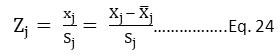
Where,
Sj = the standard deviation of Xj
Xj = the actual values of parameters
Xj = the mean of the selected parameters
To transform the data into a standardized space, the principal component analysis-based factor analysis model is now employed as Eq. 25.
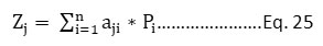
Where, j = 1,2….n
Pi = ith principal component
aji= factor loading of the jth variable on the ith principal component.
The factor loading is the jth component of the ith eigenvector of the correlation matrix multiplied by the square root of the corresponding eigenvalues. The principal components are given as Eq. 26.
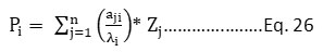
The Eigenvalues associated with Piare denoted by λi. For the determination of NAQI, the considered pollutant parameters are PM10, CO, and SO2. And the considered meteorological variables are wind speed and direction, temp. and RH.
There was a consideration of a maximum of the first three components (P1 or P1 +P2 or P1 +P2+P3), having a total variance of 60% or more. These components were calculated on the conditions that the eigenvalue should be greater than one. The NAQI was calculated by the formula given as Eq. 27, after finding the principal components (PCs),.
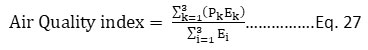
Three principal components; P1, P2, P3 are considered to have an aggregate variance of more than 60%. E1, E2, and E3 are the preliminary eigenvalues concerning the '% of variance'. Through SPSS-10.0 software, the principal components and the eigenvalues have been determined. In every principal component, the factor loading (aji) signifies the weight of each variable. The high value of factor loadings (0.70 ≤ aji< 0.99) of variables gives an idea about the most important parameter in the AQI, which indicates the degree of pollution levels.
Since there are no guidelines available for characterization of the environment in terms of 'Good', 'Moderate', 'Unhealthy', etc. associated with the values of pollution indices determined from factor analysis employed in the present study, it is not possible to draw conclusive inferences about the air-quality in absolute terms. To overcome these limitations, an approach, which involves a comparison between factor analysis-based AQI and the USEPA-based AQI, had been adopted. The variation of the pollution index with time showed a trend similar to the one exhibited by the pollution index derived from the USEPA method. However, after the inclusion of meteorological parameters into the composite index, AQI, the observed trend was very different. A significant difference between NAQIand US EPA AQI was observed. Though, when NAQI and US EPA AQI values were plotted against time, both index values followed the same trend line. The index value obtained by the factor analysis method was always less than the index value obtained by the US EPA method during air monitoring duration. NAQI shows a wider range, suggesting that it is a superior method. It is an air-stressed index without established standards. It does not show the marked effect on human health. The index is calculated by considering the synergistic effects of all selected pollutants. It can be used to relatively define the air quality status. By correlating NAQI values, air quality status at many locations can be evaluated relatively. This index can be applied to see if air quality has been worse or better throughout the months or years for all seasons by assigning a ‘Ranking,' where a higher ranking indicates higher pollution levels and vice versa.
Pollution Index (PI), 200918, 19
This index was developed by G. Cannistraro, L. Ponterio in 2009. They examined the behavior of pollutants concentrations collected every hour and daily in Messina city in 2004. Pollutants were monitored at four monitoring stations (Caronte, Archimede, Boccetta, Università) with the help of the Environment Authority of Messina. Analyzed pollutants were Respirable suspended particulate matter (PM10), benzene, CO, NO2, and O3. To formulate a new pollution index, to update people about air quality, correlation of pollutants with ambient temperature and vehicular traffic were observed. The analysis had been done to determine the relations among pollutants. The pollutants concentration levels on weekdays and weekends were also measured.
Pollutants Trends with Temperature
Correlation between pollutants concentration and temperature was studied, and it was established that ozone concentration increased with an increase in temperature and the maximum was noted during the afternoon. The highest Ozone concentration was observed during spring and summer because solar radiation is highest during that time. Ozone levels decreased from September to December, due to a decrease in ambient temperature. The concentration of Nitrogen Dioxide was decreased with an increase in ambient temperature. There was no significant comparison between major pollutants such as benzene and CO and temperature.
Pollutants Trends with Vehicular Traffic
In Messina, vehicular emissions are considered the primary source of pollution. Observing the monthly daily mean for traffic-induced pollutants, like PM10, CO, and benzene, maximum values were observed during the morning and evening peak hours, from7:30 a.m. to 8:30 a.m., and from 7:30 p.m. to 8:30 p.m respectively. Particularly, in the “University” area of Messina, the pollutants concentration values were observed maximum in three peak hours; from8:30 a.m. to 9:30 a.m., from 1:00 p.m. to 2:00 p.m., and from 7:30 p.m. to 8:30 p.m. This area has a university and court in its surrounding, so observed more traffic as compared to other areas.
Correlation Analysis
A correlation between nitrogen dioxide and tropospheric ozone was found. There was a negative correlation coefficient = -0.85 between the two pollutants. A positive correlation coefficient of 0.85 between particulate matter and nitrogen dioxide. Positive correlations were also obtained between particulate matter and benzene, carbon monoxide, and benzene respectively. The analysis revealed that there was no strong correlation between carbon monoxide and particulate matter.
The Pollution Index Method
In this index assessment of air quality is done on basis of many pollutants critical in Italian urban areas. The index represented the air quality trend in a certain urban zone. Its calculation is the mean of the two most critical pollutants’ sub-index values. The index scale is ranged from 1 to7; with increasing the number; associated risk is also increasing. The index's highest value represents the highest level of air pollution. The pollution index was calculated as per the formula represented as Eq. 28. The sub-indexes I1 and I2 were determined for the two utmost significant pollutants, presenting maximum value. The sub-indexes of the pollutants were calculated as per Eq. 29.
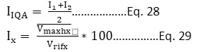
IX = Sub - index of the X pollutant
Vmax hx = Maximum concentration of X pollutant during an hour
Vrifx = Hourly limit value of X Pollutant
Table 16: Values, Indexes, and Health Risks for the PI.
|
Numerical |
Quality |
Numeric |
Health Risks |
|
0 - 50 |
Optimum |
1 |
No risks for people |
|
51-75 |
Good |
2 |
|
|
76-100 |
Moderate |
3 |
|
|
101 - 125 |
Mediocre |
4 |
Generally, there are no risks for normal people. People with |
|
126 - 150 |
Not Much Healthy |
5 |
There are risks for children, heart diseases, and olds age |
|
151 - 175 |
Unhealthy |
6 |
Many people may feel light adverse symptoms, which are |
|
>175 |
Very Unhealthy |
7 |
People may feel light adverse effects on health. There are |
General Air Quality Health Index (GAQHI), 202133
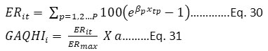
The index is constructed in Beijing, China, considering the aggregation of pollutants. In this index, it is tried to overcome the limitation of other indexing systems, and efforts are made to incorporate the cumulative effects of multiple pollutants’ exposure. The index is based on the excess risk estimation, as shown in eq. 30 and eq. 31.
Where,
βp = exposure-response relationship coefficient of air pollutant p for its expected health outcomes
ERit = Excess risk in the ith city at time t
xtp = Average 3 hrs. the concentration of pollutant p at time t
ERmax = Maximum value of ERit throughout the study period
a = standardization coefficient varies between 0 to 10, a = 10 value is recommended
GAQHIi = General air quality health index of the city i
This index cannot be applied to all the cities is the limitation of this index. As βp value is different for different cities. This index is based on the impact of pollutants on human health and considers all major pollutants simultaneously. But this index cannot be used to show real-time air quality status.
Discussion
Up to 1970, many researchers tried to develop the air quality indexing system in different countries, considering only two to three air pollutants such as SPM or COH, CO, and SO2. In 1971, the oak ridge air quality index was developed in which five pollutants (photochemical oxidants, SO2, NO2, CO, and SPM) were considered. From 1972 to 1975, there was not much research on developing air quality indexing systems. Then in 1976, US EPA suggested an index which was known as pollutant standard index (PSI). This index is based on maximum operating function and is widely used by many countries. Again there was no significant development in the air quality indexing system from 1977 to 1992, and from 1994 to 1998. In 1993, two indexing systems were developed: i. Integral air pollution index (IAPI) which was based on maximum permissible concentration and developed for Russian cities, ii. A simple air quality index was developed for Finland which was based on linear interpolation and maximum operating function but considered WHO standards as breakpoint concentration. In 1999, US EPA modified the air quality index. The name changed from pollutant standard index (PSI) to air quality index (AQI). Instead of TSPM, PM10 and PM2.5 were incorporated in the calculation of AQI, and breakpoint values of pollutants were modified. In 1999, Swamee and Tyagi also developed an aggregate index.
After almost four years in 2004, two indexing systems: i. Revised air quality index (RAQI), and ii. A pollution index (PI) was developed. RAQI is based on entropy function and is more useful to predict long-term health impact and long-term air quality. The pollution index (PI) was developed for the city of Itlay. It is a modified version of US EPA AQI, in which European standards were considered in breakpoint values of pollutants. Murena et. al. developed the pollution index by considering maximum operating function as well as synergetic effects of pollutants. Based on the results obtained it was concluded that additive effects of pollutants strongly influenced the air quality evaluation. In 2006, the air quality depreciation index was developed which is based on value function graphs, and the index measures the deterioration in air quality. In 2007, two different air quality indexing methods were developed: i. An aggregate air quality index, and ii. CITEAIR’s Common air quality index (CAQI). An aggregate air quality index was developed by George Kyrkilis et.al. for the Athens city, and also compared this index with US EPA-based AQI. Based on the comparison the researcher concluded that the aggregate index estimated more effectively the impacts of the pollutants to the population as contrasted to US EPA-based AQI. The CAQI under the CITEAIR project was developed for European cities which is based on the US EPA formula. This index also showed a significant difference between city background stations and traffic stations. In 2009, two indexing systems were developed: i. New air quality index (NAQI), and ii. Pollution index (PI). Principal component analysis (PCA) and factor analysis based on the new air quality index (NAQI) was developed in India. It was developed to incorporate the deficiencies of USEPA based AQI. The index developer also developed the NAQI with US EPA-based AQI. The comparison between the two indexing systems concluded that when NAQI and US EPA AQI values plotted against time, both index values followed the same trend lines, but when meteorological parameters were incorporated in NAQI, vast differences were observed between the two trend lines. The NAQI values were always less than the US EPA values, but NAQI values were in a wider range proved superiority. The sub-index of the pollution index is the ratio of hourly pollutant concentration to its corresponding standards. It was calculated by taking the average of the two most critical pollutants’ sub-index values. From 2010 to 2017, there is a development of a fuzzy-based air quality indexing system. In 2021, a human health impact-based general air quality health index is developed in Beijing, China. But this index cannot be used universally.
A fuzzy logic system is very suitable for addressing subjective environmental issues, which usually involve a degree of uncertainty. The fuzzy sets theory is very helpful in handling the uncertainty in the assessment of air quality. Keeping the importance of flexibility of the fuzzy sets theory in an imprecise environment and the decision-making process, many researchers tried to develop the fuzzy-based air quality indexing systems, which are reviewed and compiled in separate section 3.
Evolution of Fuzzy Based Air Quality Indexing System
Air Pollution Monitoring Using Fuzzy Logic, 201020
The authors applied a real-time fuzzy logic system using Simulink to calculate AQI. The fuzzy logic control process consisted following steps: i. Defining the input variables - they used five pollutants as input variables; SO2, NO2, PM10, O3, and CO. In this step, pollutants are categorized into five groups; good, moderate, poor, very poor, and severe based on their respective standards, ii. Fuzzification: it is the process to transform crisp values into membership grades for fuzzy sets language. In the fuzzy logic process, fuzzification is the first step in which the crisp inputs are converted to fuzzy inputs by determining the membership function for each point. iii. Fuzzy inference rules: in which, the information related to the given problem is expressed as a set of fuzzy inference rules. iv. Defuzzification: in the MATLABFLC module, to get a crisp output, the center of gravity method is used. The authors applied their suggested model to compute AQI and concluded that the model produce acceptable simulation outcomes.
Fuzzy Synthetic Evaluation Model Based Air Quality Index (FAQI), 201423
TheFAQI is calculated by bearing in mind the weights of all selected pollutants and accumulating the pollutants. They considered the four pollutants; SPM, RSPM, SO2, and NO2. Since air pollutants have different severity on the health of human beings, their weights were considered different in FAQI. The weight of individual pollutants was determined through an analytical hierarchical process (AHP). The researcher attempted to combine the analytical hierarchical process (AHP) and fuzzy synthetic evaluation model for risk assessment of air pollution. The main characteristics of fuzzy logic are its uncertainty, which can be quantified by fuzzy sets theory.
The authors collected the air quality data of four monitoring stations of the Taj Trapezium zone for the year 2011 – 12 from the CPCB. They developed the fuzzy model based on the pollutants concentrations range, given in the AQI system, India developed by Sharma et. al. in 2003. The index is classified into five levels: very good to very poor, and in between three levels: good, moderate, and poor. These categories were defined as five risk levels to characterize the air quality class in the fuzzy model. AQI values and their corresponding pollutants concentration are tabulated in Table – 17.
Table 17: AQI and Corresponding Breakpoint Concentration.
|
Pollutants |
AQI categories and corresponding breakpoint concentrations |
||||
|
|
0 -100 |
101 -200 |
201 -300 |
301-400 |
401- 500 |
|
SPM (ug/m3) |
0 -200 |
201-300 |
301 -700 |
701 -840 |
841-1200 |
|
RSPM (ug/m3) |
0 -100 |
101 - 150 |
151 -350 |
351-420 |
421- 500 |
|
S02, (.ijg/m3) |
0 -80 |
81 -367 |
368 -786 |
787 - 1,572 |
1,573 -2,000 |
|
:t:l.Q.. (ugtm3) |
0 - 80 |
81 - 180 |
181 - 564 |
564 - 1,272 |
1,273 - 1,500 |
The breakpoint concentration values were categorized as representative values (ei) in the creation of a fuzzy design recognition model. The standard values (NAAQS, India, 1994, 2009) for the sensitive zone were used as the benchmark values (pi) as the model was developed for the air quality assessment of the Taj Trapezium Zone, which is classified as the sensitive zone. The membership degree of FAQI ranged from 0 to 1. For all pollutants, the worst air quality is represented by the membership degree 1 i.e. FAQI value is 6, while the clean air is represented by the membership degree 0 i.e. FAQI value is 1. For FAQI, the authors determined a scale of 1 to 6. The scale 1 – 2, 2 – 3, 3 – 4, 4 – 5, and 5 -6 is rated as very good to very poor as defined by Sharma et. al.
Relative Weights of Air Pollutants
Concerning the health impact, each pollutant parameter has different importance and hence, different weights are attributed. The AHP can be used to determine the weighing of individual pollutants. In AHP, a pair-wise comparison matrix A is formed as given below, where the number in the ith row and jth column gives the relative importance of individual air pollutant Pi as compared to Pj.
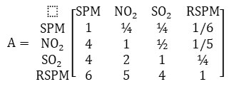
In this case, the authors gave 6 times more weightage to RSPM as compared to SPM and 4 times more weightage to NO2 and SO2 as compared to SPM. They gave 2 times and 5 times more weightage to SO2 and RSPM respectively as compared to NO2 and gave 4 times more weightage to RSPM as compared to SO2.
The normalized weights were calculated by dividing each cell by the column sum. The obtained normalized weight matrix N:
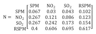
The pollutants’ relative weight was determined by calculating the mean value of each row of matrix N. The relative weight matrix W:
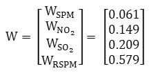
Thus, the sum of the weighing of the pollutants obtained as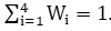 . The data analysis revealed that the SO2 and NO2 concentrations were always within permissible values in all four monitoring locations. While at all four monitoring locations, RSPM and SPM concentration have exceeded the standards, most of the days. The authors observed that in winter, the concentration levels were found to be higher as compared to the summer season because of meteorological parameters.
Using a fuzzy synthetic evaluation model, for four monitoring stations, the FAQI values were determined. The determined index value indicates that at all the monitoring locations, air quality is poor in December and January and FAQI values mainly lay in the poor and moderate category. For the permissible concentration levels, the calculated FAQI values were two. The results show that the FAQI values for monitoring data exceeded the permissible FAQI value in most of the days.
Fuzzy Based Air Quality Health Index (FAQHI) - An Innovative Approach, 201532
The FAQHI was calculated by using fuzzy – AHP. In the determination of FAQHI, five pollutants; PM10, NO2, SO2, O3, and CO together with three subjective parameters; population density and sensitivity, and location sensitivity were considered. The FAQHI was applied to Howarh city, India for the year 2009 to 2011. In the determination of the index, different weights were assigned to pollutants and subjective parameters. To determine the weightages of the pollutants and subjective parameters, a fuzzy pair wise comparison matrix was developed, in terms of pollution index (PI) and exposure index (EI) respectively. The FAQHI matrix considered the pair-wise comparison between the PI matrix and EI matrix. For defining the uncertainty range, α cut was introduced in pollution index matrix, exposure index matrix, and FAQHI matrix and all three matrices were converted to fuzzy pollution index matrix (PIf), fuzzy exposure index matrix (EIf), and FAQHIf respectively. The PIf, EIf, and FAQHIf matrix converted to crisp comparison (PI’, EI’, and FAQHI’) matrix using eq. 32.
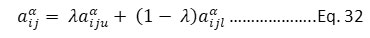
Where,
aiju and aijl = upper and lower value of comparison element,
λ = 0.5
The software MATLAB 7.10.0 was used to calculate the eigenvalues and eigenvectors from crisp matrices. Normalization of eigenvectors was done to determine the local weights of individual parameters, represented as PIw, EIw, and FAQHIw. Local weights are applied to determine the aggregate weights of different parameters. The triangular fuzzy membership function was used to determine the fuzzy membership function. After establishing the membership degree matrix (R), the defuzzification process was done. The advantage of this index is that it considered multi-pollutant parameters with subjective parameters. The index is helpful to estimate the health impact considering air quality as well as other local conditions.
Air Quality Indices using Fuzzy Logic: Feasibility Analysis, 201621
The researchers collected the air pollutant concentrations at industrial, residential, and sensitive areas of Bangalore. Three pollutants; RSPM, NO2, and SO2 have been collected over six sites of Bangalore. Out of these, three sites were in the industrial zone, two sites were in a residential zone, and one site was in a sensitive zone. The data regarding pollutants concentration were obtained from, “Karnataka State Pollution Control Board (KSPCB), Bangalore” for the duration of five years; 2008 – 2013. The Air Quality Indexes were calculated through linear interpolation formula and maximum operating function. The authors used a real-time fuzzy logic system with Simulink to compute AQIand reported that this system gives agreeable results. This system can also work under the continuous working mode, efficiently. The authors concluded that the AQI model based on fuzzy rules is a powerful tool to suggest to human beings about outdoor activities in a particular area. They also observed that the results obtained through the fuzzy approach were more efficient than the linear interpolation approach.
Fuzzy Inference System Based Air Quality Indices, 201722
The authors used a Mamdani fuzzy inference system-based model to assess the air quality of Chennai. They considered three pollutants; SO2, NO2, and RSPM. Data were collected from the Tamilnadu SPCB, Chennai for the year 2007 to 2015. Four sampling stations, two in a commercial area, one in an industrial area, and one in a residential area were selected. The authors determined the membership function and fuzzy inference rules based air quality index. It was concluded that the results obtained through the fuzzy rules system were better than the results obtained through other methods.
Discussion
The AQI system based on fuzzy logic has been evaluated since 2010. The fuzzy-based AQI is more reliable than the other methods. Out of all the above describing methods, fuzzy synthetic evaluation-based AQI and fuzzy air quality health index are more powerful tools to describe the air quality.
Air Quality Indexing Systems Existing in India
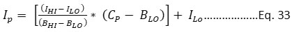
In India, presently two indexing systems prevail, i. Air Quality Index for India, and ii. National Air Quality Index, India. Both indexing systems are based on the US EPA formula and maximum operating function as shown in Eq. 34. As indicated in Eq. 33, for pollutant concentration (Cp), the sub-index (Ip) is determined using the "linear segmented concept."
Where,
Ip = Sub-index of pollutant P
AQI = Max (IP) ……………Eq. 34
Where,
P = 1,2,3………, n; denotes n pollutants
Because the maximum operating function is devoid of eclipsing and ambiguity, it is used. Due to simplicity in maximum operating function, it is adopted by many countries. Both the indexing systems are studied in-depth and summarized as sub-section 4.1 and 4.2.
Air Quality Index for India, 201034
The air quality index for India was developed by IITM, Pune with the assistance of MoES as part of the SAFAR project in August 2010. The SAFAR project can predict the air quality for the next three days. This indexing system has been implemented in four cities: Delhi, Mumbai, Pune, and Ahmedabad. The SAFAR – AQI system considered five pollutants: PM2.5, PM10, NO2, CO, andO3. The index range is from 0 to 500 and is distributed into six categories, from good to severe. The AQI categories and pollutants breakpoint values are shown in Table 18.
Table 18: IITM-SAFAR Air Quality Descriptors, AQI Values, and Corresponding Air Pollutants Breakpoint Values.
|
AQI Category (Range) |
PM10 |
PM2.5 |
NO2 |
O3 |
CO |
|||||||
|
|
Ilow |
Ihigh |
Clow |
Chigh |
Clow |
Chigh |
Clow |
Chigh |
Clow |
Chigh |
Clow |
Chigh |
|
Good |
0 |
50 |
0 |
50 |
0 |
30 |
0 |
21 |
0 |
25 |
0 |
0.9 |
|
Satisfactory |
51 |
100 |
51 |
100 |
31 |
60 |
22 |
43 |
26 |
51 |
1 |
1.7 |
|
Moderately Polluted |
101 |
200 |
101 |
250 |
61 |
90 |
44 |
96 |
52 |
86 |
1.8 |
8.7 |
|
Poor |
201 |
300 |
251 |
350 |
91 |
120 |
97 |
149 |
87 |
106 |
8.8 |
14.8 |
|
Very Poor |
301 |
400 |
351 |
430 |
121 |
250 |
150 |
213 |
107 |
381 |
14.9 |
29.7 |
|
Severe |
401 |
500 |
431 |
700 |
251 |
380 |
214 |
750 |
382 |
450 |
29.8 |
40 |
National Air Quality Index (NAQI), 20142
For the development of NAQI, CPCB has assigned the work to IIT - Kanpur. The index was launched in October 2014. An AQI's goal is to swiftly communicate news about real-time air quality. Eight Pollutants; PM2.5, PM10, SO2, NO2, O3, CO, NH3, and Pb having short-term norms have been studied. A scientific basis for meeting air quality standards, as well as dose-response relationships for specific pollutants, has been created and used to determine breakpoint values for each AQI class. Table 19 shows the air quality index categories with breakpoint values of pollutants.
Table 19: Breakpoint Values of Pollutants for NAQI.
|
AQI Category |
PM10 |
PM2.5 |
NO2 |
O3 |
CO |
SO2 |
NH3 |
Pb |
|
Good (0-50) |
0-50 |
0-30 |
0-40 |
0-50 |
0-1.0 |
0-40 |
0-200 |
0-0.5 |
|
Satisfactory |
51-100 |
31-60 |
41-80 |
51-100 |
1.1-2.0 |
41-80 |
201-400 |
0.6-1.0 |
|
Moderate |
101-250 |
61-90 |
81-180 |
101-168 |
2.1-1.0 |
81-380 |
401-800 |
1.1-2.0 |
|
Poor |
251-350 |
91-120 |
181-280 |
169-208 |
10.1-17 |
381-800 |
801-1200 |
2.1-3.0 |
|
Very Poor |
351-430 |
121-250 |
281-400 |
209-748* |
17.1-34 |
801-1600 |
1201-1800 |
3.1-3.5 |
|
Severe |
430+ |
250+ |
400+ |
748+ |
34+ |
1600+ |
1800+ |
3.5+ |
*One hourly monitoring (for mathematical calculation only)
Discussion
The study of existing air quality indexing systems in India revealed that both indexing systems are based on maximum operating function and linear segmented principles. SAFAR-IITM AQI is implemented only in four metropolitan cities and considered only five pollutants. While NAQI has been adopted by CPCB and implemented in the whole country. During the development of NAQI eight criteria pollutants having short-term impacts have been considered. And the breakpoint values of the pollutants have been decided based on the impact of the pollutants on human health or the breakpoint values adopted by the US EPA.
Conclusion
From all the indexing systems listed above from 1966 to 202021, it can be concluded that there are always some drawbacks and no system is entirely perfect. Attempts should be made to evolve the indexing system for the region because each area is different geographically and the index which may apply to one area may or may not apply to another. All the characteristics for the area should be carefully considered, major pollutants should be considered and only then the system should be finalized. An ideal indexing system is a system that is expandable, unambiguous, free from eclipsing, and understandable by a layman. Indexing should not be based on the maximum operating function, as this system does not reflect that whether more than one pollutant exceeded the standards or not. The ideal indexing system should consider the aggregation and synergetic effects of pollutants. It should be based on community data available from the local monitoring system, an arrangement shall be made such that in hazardous conditions an alarm is generated so that citizens are made aware. Integration of all the above-stated indexes can be done to develop a global index,which not only helps to compare air quality but also protect the citizens from deteriorating air quality. When compared with other methods, the AQI system based on fuzzy logic is a more powerful instrument that produces more consistent findings. But till 2017, there is no development of a fuzzy-based AQI system in which fine particulate matter (PM2.5) has been considered. So, there is a need to develop the fuzzy-based air quality indexing system considering PM2.5 as a pollutant with other air pollutants.
Acknowledgment
The first author is thankful to CEPT University for allowing her to do the Ph. D. research work. The authors would also like to thank all the air quality index developers for their work. Based on their work only, a compilation of the evolution of the air quality indexing system could be possible.
Funding Source
The authors received no financial support or any type of funding for this research work, authorship, and/or publication of this research article.
Conflict of Interest
The authors do not have a conflict of interest to declare including any financial, personal, or other relationships with other people or organizations that can influence the work.
References
- Green MH. An Air Pollution Index Based on Sulfur Dioxide and Smoke Shade. Journal of the Air Pollution Control Association. 1966; 16(12):703-706.doi:10.1080/00022470.1966.10468537.
CrossRef - https://app.cpcbccr.com/ccr_docs/FINAL-REPORT_AQI_.pdf
- Atmakuri K, Anandam D, Srinivasu D. A Survey Paper on Spatial-Temporal Outliers Influencing Air Quality. International Journal of Engineering Research and Development. 2018; 14(1):39-43. Accessed July 8, 2021. http://www.ijerd.com/paper/vol14-issue1/Version-2/G140123943.pdf
- Shenfeld, L. (1970). Ontario’s air pollution index and alert system. Journal of the Air Pollution Control Association, 20(9), 612-612.
CrossRef - Fezari, M., Hattab, R., & Al-DAahoud, A. (2015). Oak Ridge Air Quality Index Computation: a way for Monitoring Pollutions in Annaba City. In Conference: International Arab Conference on Information Technology (ACIT).
- Wayne R. Ott & William F. Hunt, Jr. (1976) A Quantitative Evaluation of the Pollutant Standards Index, Journal of the Air Pollution Control Association, 26:11, 1050-1054.
CrossRef - Bezuglaya, E. Y., Shchutskaya, A. B., & Smirnova, I. V. (1993). Air pollution index and interpretation of measurements of toxic pollutant concentrations. Atmospheric Environment. Part A. General Topics, 27(5), 773-779.
CrossRef - Kanchan, Kanchan, Amit Kumar Gorai, and Pramila Goyal. "A review on air quality indexing system." Asian Journal of Atmospheric Environment 9.2 (2015): 101-113.
CrossRef - Hämekoski, K. (1998). The use of a simple air quality index in the Helsinki area, Finland. Environmental Management, 22(4), 517-520.
CrossRef - Cheng, W. L., Chen, Y. S., Zhang, J., Lyons, T. J., Pai, J. L., & Chang, S. H. (2007). Comparison of the revised air quality index with the PSI and AQI indices. Science of the Total Environment, 382(2-3), 191-198.
CrossRef - Swamee, P. K., & Tyagi, A. (1999). Formation of an air pollution index. Journal of the Air & Waste Management Association, 49(1), 88-91.
CrossRef - Cheng, W. L., Kuo, Y. C., Lin, P. L., Chang, K. H., Chen, Y. S., Lin, T. M., & Huang, R. (2004). Revised air quality index derived from an entropy function. Atmospheric Environment, 38(3), 383-391.
CrossRef - Murena, Fabio. (2004). Measuring air quality over large urban areas: Development and application of an air pollution index at the urban area of Naples. Atmospheric Environment. 38. 6195-6202. 10.1016/j.atmosenv.2004.07.023.
CrossRef - Singh, G. (2006). An index to measure depreciation in air quality in some coal mining areas of Korba industrial belt of Chhattisgarh, India. Environmental monitoring and assessment, 122(1), 309-317.
CrossRef - Kyrkilis, G., Chaloulakou, A., & Kassomenos, P. A. (2007). Development of an aggregate Air Quality Index for an urban Mediterranean agglomeration: Relation to potential health effects. Environment International, 33(5), 670-676.
CrossRef - Léger K, Nussio F, Cagnoli M, et al. Comparing Urban Air Quality in Real Time the CITEAIR Common Air Quality Index (CAQI) for Europe. ; 2006. Accessed July 8, 2021. http://citeair.rec.org/downloads/caqi_20_march_2006.pdf.
- Bishoi, B., Prakash, A., & Jain, V. K. (2009). A comparative study of air quality index based on factor analysis and US-EPA methods for an urban environment. Aerosol and Air Quality Research, 9(1), 1-17.
CrossRef - Cairncross, E., John, J., & Zunckel, M. (2003). Methodology for developing an air pollution index (API) for South Africa. Clean Air Journal= Tydskrif vir Skoon Lug, 13(2), 19-29.
CrossRef - Cannistraro, G., & Ponterio, L. (2009). Analysis of air quality in the outdoor environment of the city of Messina by an application of the pollution index method. Int J Civ Environ Eng, 1(4), 214.
- Upadhyaya, G., & Dashore, N. (2010). Monitoring of air pollution by using fuzzy logic. International Journal on Computer Science and Engineering, 2(07), 2282-2286.
- Lokeshappa, B., & Kamath, G. (2016). Feasibility analysis of air quality indices using fuzzy logic. Int. J. Eng. Res. Technol, 5(8).
CrossRef - Swarna, E., and M. Nirmala. "Analysis of air quality indices using fuzzy inference system." 2017 IEEE International Conference on Smart Technologies and Management for Computing, Communication, Controls, Energy, and Materials (ICSTM). IEEE, 2017.
CrossRef - Gorai, A. K., Upadhyay, A., & Goyal, P. (2014). Design of fuzzy synthetic evaluation model for air quality assessment. Environment Systems and Decisions, 34(3), 456-469.
CrossRef - Van den Elshout, S., Léger, K., & Nussio, F. (2008). Comparing urban air quality in Europe in real-time: A review of existing air quality indices and the proposal of a common alternative. Environment International, 34(5), 720-726.
CrossRef - Stieb, D. M., Burnett, R. T., Smith-Doiron, M., Brion, O., Shin, H. H., & Economou, V. (2008). A new multipollutant, no-threshold air quality health index based on short-term associations observed in daily time-series analyses. Journal of the Air & Waste Management Association, 58(3), 435-450.
CrossRef - Sicard, P., Talbot, C., Lesne, O., Mangin, A., Alexandre, N., & Collomp, R. (2012). The aggregate risk index: an intuitive tool providing the health risks of air pollution to the health care community and public. Atmospheric environment, 46, 11-16.
CrossRef - Kyrkilis, G., Chaloulakou, A., & Kassomenos, P. A. (2007). Development of an aggregate Air Quality Index for an urban Mediterranean agglomeration: Relation to potential health effects. Environment International, 33(5), 670-676.
CrossRef - Kumar, A., & Goyal, P. (2013). Forecasting of air quality index in Delhi using neural network based on principal component analysis. Pure and Applied Geophysics, 170(4), 711-722.
CrossRef - Mandal, T., Gorai, A. K., & Pathak, G. (2012). Development of fuzzy air quality index using soft computing approach. Environmental monitoring and assessment, 184(10), 6187-6196.
CrossRef - Gorai, A. K., Upadhyay, A., Tuluri, F., Goyal, P., & Tchounwou, P. B. (2015). An innovative approach for the determination of air quality health index. Science of the Total Environment, 533, 495-505.
CrossRef - SAFAR-Ahmedabad & Ahmedabad-AIR plan dedicated to the Nation by Hon. Minister, MoES. www.tropmet.res.in. Accessed July 7, 2021. https://www.tropmet.res.in/74-event_details
- Gorai, Amit Kumar, et al. "An innovative approach for determination of air quality health index." Science of the Total Environment 533 (2015): 495-505.
CrossRef - Tan, Xiaorui, et al. "A review of current air quality indexes and improvements under the multi-contaminant air pollution exposure." Journal of environmental management 279 (2021): 111681.
CrossRef - M. Gurfan Beig, IITM, “SAFAR, AQI,” 2010. http://safar.tropmet.res.in/AQI-47-12-Details (accessed Nov. 30, 2021).


