Current World Environment

Introduction

Particulate matter pollution and increase in carbon dioxide concentration are seen as the major troubles man is facing today with respect to health and the environment. In 2016, the health effect institute (IHE) noted that the chronic exposure to ambient PM_2.5 killed about 4.1 million people and caused a disability-adjusted life years’ (DALYs’) loss of 106 million; the highest total deaths were obtained in India (25%) and China (26%).¹ These data were obtained by the extensive air quality monitoring network stations in urban areas of developed countries and the satellite observation of air quality combined with obtained information from models of global chemical transport to estimate the global PM_2.5­ concentration and its consequent effects on humans.¹ PM_2.5 originates from fossil fuel combustion in power plants, congested traffic flow, and heating from residential and industrial areas using oil, coal, or wood.² PM₁₀ has a detrimental effect on human health by its blocking and destructive effect on the nasal and bronchial passages, igniting different respiratory-related effects that end up in sickness or death.³ PM₁ consists of anthropogenically derived particles having dangerous impacts on the human respiratory and cardiovascular systems by directly entering the blood system⁴. Very small particles (<1μm) pass into the lungs and then the bloodstream via the blood barriers and cause some severe health complications.⁴ One of the major concerns related to air in today’s scenario is the increasing concentration of carbon dioxide and its role in the environment. Atmospheric CO­₂ has been increasing by ? 3 ppm/year since 2001 and can be attributed to the increase in the global use of fossil fuels, particularly in China and India.⁵ The situation of Kashmir is no different from that of other parts of India and the world. Even Srinagar city is exhibiting increased concentrations of particulate matter and CO₂ due to industrialization and increased vehicular population.⁶ The ambient concentrations of particulate matter and carbon dioxide caused by vehicular pollution were monitored from 2019 to 2020 in Srinagar city and the findings showed that during the whole period, average PM₁ concentrations ranged from 15.10 -108.9 μg/m³, PM_2.5 (28.70 -577.50 μg/m₃), PM₄ (44.50 -780.87 μg/m³), PM₁₀ (57.13-1225.53 μg/m³), TSP (77.77-1410.27 μg/m³) and CO₂ (332.4 - 655.0 ppm).⁷

The Inverse Distance Weighting (IDW) technique of spatial interpolation that is available in geospatial tools like the QGIS, ArcGIS, etc. estimates cell values by weighting values of geometric data in the neighborhood of each processed cell. In the weighting process, the points situated nearer to the cell center have more influence or weight on the processed cell.  This technique assumes that as distance increases from the sampling site, the influence of the entered variables on the maps decreases with respect to the sampling site.⁸ The inverse distance weighting has been proven as the finest technique for the interpolation of air quality assessment data in urban delicate zones.⁹ It has also been proven to produce a better comparison between interpolated and measured values of suspended particulate matter, SO_2, and NO₂ than Kriging during an appraisal of different techniques of interpolation for the parameters of the ambient air quality of Port Blair.¹⁰ The IDW was a very necessary tool to figure out the relations between health effects and air pollution in the assessment of the daily trend of PM_2.5 concentration for the contiguousness of the United States from 2009, at county and census block group levels respectively.¹¹ It was also used to measure and interpolate the concentration of the aerosol optical thickness (AOT) at 40 locations in the areas of urban Ranchi and to quantify the conditions of the atmosphere at 42 locations in the coalfield zones of Southern Karanpura.¹² The primary use of interpolation techniques has been to map out bedrocks, soils, air quality assessment, and ground and surface water studies.^13,14 Since the inverse distance weighting has such important usefulness in interpolating and mapping air quality parameters, and since no such work has been published for Srinagar city nor given much attention to the in-depth/systematic study of its air quality and the responsible factors for its deterioration¹⁵, this paper presents six months study IDW maps of the spatial variation and interpolation of particulate matter and carbon dioxide for an idea of the pollutant blanket over the city using some tourists’ locations as sampling/monitoring sites.

Materials and Methods

Study Area

Srinagar city located at N 34.08^o, N 74.80^o in the Kashmir valley is internationally known for its remarkable gardens and lakes. The stunning looks of the gardens in Srinagar have attractive hill slides, flowering shrubs and trees, and enthralling water bodies. Notwithstanding the witness of centuries of change, the gardens still attract tourists from all over the world. The study area shown in Figure 1 includes Chesmashahi Botanical Garden (N 34.09^o, E 074.87^o), Nishat Garden (N 34.12^o, E 074.88^o), Naseem Bagh (N 34.14^o, E 074.84^o), Harwan Garden (N 34.16^o, E 074. 90^o), Shalimar Garden (N 34.14^o, E 074.87^o), Lal Chowk (N 34.07^o, E 076.81^o) and Sher-e-Kashmir University of Agricultural Sciences and Technology of Kashmir (SKUAST-K) Shalimar campus (N 34.15^o, E 074.88^o). The areas that experience more traffic are Lal Chowk, Naseem Bagh, Nishat Garden, and Shalimar Garden. Those that experience less traffic are Chesmashahi Botanical Garden, Harwan Garden, and SKUAST-K Shalimar campus.

Figure 1: Digital Map of the Ambient Air Monitoring Sites/Locations. Click here to view Figure

Ambient Air Monitoring Method

The Aerocet 831-Aerosol Mass Monitor and CDM 901-CO₂ Monitor were used every fortnight to monitor the ambient concentrations of particulate matter and carbon dioxide respectively in the morning, afternoon, and evening for a triplicate sampling data for a period of six months from November 2019 to April 2020. Both instruments were held away from disturbances like vehicular movements and human gatherings for about one minute at some height to record the data of particulate matter (PM₁, PM_2.5, PM₄, PM_10, and TSP) and carbon dioxide respectively. The Aerocet 831-Aerosol Mass Monitor is a small-handheld instrument that operates on a battery for measuring the mass of particulate matter in the ambient air. It weighs about 0.79 kg and can be used for up to 24 hours for intermittent sampling. This instrument has a sensitivity that ranges from a high of 0.3 μm to a low of 0.5 μm and thus monitors the levels of PM₁, PM_2.5, PM₄, PM_10, and TSP simultaneously ¹⁶. The provision of simple and efficient operation is due to the many functions of the rotary dial. It has the capacity of differentiating seven ranges of particles by counting and sizing them and then converting the counted data to mass measurement (µg/m³) by using a proprietary algorithm. It computes for each particle detected a volume then allocates for the transformation a standard density value which is improved by the setting of a K-Factor to make a better measurement accuracy of ±10% to calibration aerosol.¹⁶ A Comet software which is a program that extracts information (alarms, data, settings, etc.) from Met One Instruments’ products¹⁷ modifies these K-Factors which, with a reference unit can be analytically obtained. Or a recommended K-Factor setting of 3.0 is used in the case of an unavailable reference unit. This instrument uses the operating principle of particle count to mass conversion using scattered laser light.¹⁸ As the particles enter via the detection chamber which contains a photodetector and samples one particle at a time, the laser light is scattered and detected by the photodetector. The instrument can analyze the scattered light’s intensity and deduce the particle’s size. In addition, the number of received lights on the photodetector can be used by the instrument to account for the number of particles in the detection chamber. This approach is advantageous because it can use a single detector/analyzer to simultaneously sense different diameter particles.

Whereas, the CDM 901- CO₂ monitor works with the principle of NDIR (Non-Dispersive Infrared Radiation), and the NDIR sensors functions on the principle of the absorption of infrared radiation (IR) by a particular gas. The sensor becomes sensitive to a certain gas because of the usage of different bands of absorption in the infrared spectra. At the wavelength of 4.3 μm, carbon dioxide strongly absorbs IR radiation, thereby avoiding the bands 2.5 to 2.9 and 5.2 to 7.5 μm at which water vapor is absorbed.¹⁹ The path length of the IR that is between the detector and the source orders the gas level the sensor can detect and the Beer’s Law, I = I_o exp (-α ?) describes the relationship. From the above formula, the transmitted light via the gas cell is I  and the incident light on the gas cell is I_o, the sample’s absorption coefficient (cm^-1 units) is given as α and the optical pathlength of the cell is given as ?.²⁰ As pathlength increases, the signal that is received and the infrared radiation’s intensity exponentially decreases with it. The infrared detector produces a higher signal as path length decreases. But, there’s a decrease in sensitivity, since a shorter optical path reduces the gas’ absorption distance for the radiation.²¹ The range of CDM 901 is from 0-2000 ppm. The resolution stands at 1% of the full scale i.e., 20 ppm. The sampling is done by diffusion technique without the need for a pump. The response time for the reading is less than 15 seconds. The inbuilt LCD shows the humidity and temperature range of the ambient air along with the CO₂ concentrations.²¹

Preparation of IDW Maps of Particulate Matter and CO₂ Concentrations

The inverse distance weighting (IDW) obtainable in QGIS software version 3.16.3 was used to map out the concentration of particulate matter (PM) and carbon dioxide (CO₂) by the interpolation of data generated at the seven (7) monitoring sites. To predict the concentration of pollutants for locations in which sampling was not done, the IDW interpolates the data obtained for the sampled location assuming that areas closer to each other are similar than those farther apart.²² On each map, a pollutant was interpolated on monthly basis for the six months of monitoring to show the pollutant’s spatial variability in the nearby areas of the sampling locations where sampling was not undertaken. Unknown values/concentrations of geographic parameters such as elevation, chemical concentrations, and noise levels of places that are hard, costly, or even impossible to access have been predicted by interpolation techniques with few data for sampled areas/points.^23,14 Flexibility for carrying out interpolations that are efficient and optimal for the spatial variation of any given number of samples is provided by the IDW interpolation technique^4,24,14 The prediction of the concentration of the pollutants in the nearby locations was done by observing the ten (10) partitions by which the maps were scaled.

Statistical Analysis

On the fortnight of each month, three replications for each sampling/monitoring site were taken and the average triplicate data obtained for each month and the average six months of monitoring pollutants load at the seven locations were analysed using the R software version 4.0.4. A one-way analysis of variance (ANOVA) of the randomized complete block design (RCBD) is an experimental design for comparing treatments in blocks with homogenous experimental units was used for the analysis in the R software to get the critical difference (CD) of significance at p ≤ 0.05 to determine the monthly and average six months variation (significant or insignificant) of the pollutants among the different monitoring locations respectively. Also, the average data of the monitored pollutants for the six months of sampling were subjected to a Pearson correlation matrix analysis to know their pattern in a relationship (positive or negative and significant or insignificant).

Results and Discussion

The data in Table 1 shows the monthly mean variation of each monitored parameter at the study sites that were interpolated on monthly basis using the Inverse Distance Weighting (IDW) technique in the QGIS software version 3.16.3.

Table 1: Monthly Variation of Particulate Matter and Carbon Dioxide at the Different Study Sites/Monitoring Locations.

Critical Difference (CD) is significant at p ≤ 0.05; SE(d) is the standard error of the difference

The Inverse Distance Weighting (IDW) maps (Figure 2 – 7) show the interpolation of the variation of the concentration of the monitored pollutants at the sampling sites to the unsampled locations in each month to predict the concentration values of the monitored pollutants for the unsampled locations. These maps significantly show that the concentrations of pollutants decrease with distance from their respective sampling sites. Thus, the assumption is that each monitored sampling site has an influence locally that diminishes with distance. On each map, the thick red domains represent the areas with the highest concentration of the pollutants which fades out with distance showing a decrease in the concentration of pollutants with an increase in distance from the study site. The thick blue domains characterize the zones with the lowest concentration of pollutants. The legend on each figure in a descending order i.e., from dense blue to dense red, shows an increase in the concentration of pollutants; and in ascending order i.e., from thick red to thick blue, shows a decrease. The influence of pollutants on the different nearby locations can be predicted based on how far the scaling area covers the coordinates on the map. The major objective of the investigation is to come up with simple but inclusive maps that show and predict an estimate of the variation and blanket of the monitored pollutants respectively over the city to get an immediate requirement of estimation of pollutants at different sites in Srinagar due to the homogeneity in topography.

Table 1 (a and b) and Figs. 2 and 3 show the data and IDW maps of the monthly spatial variation of PM₁ and PM_2.5 at the monitoring sites respectively.  The data and IDW maps show that in each month there was a significant monthly spatial variation of the concentrations of PM₁ and PM_2.5 between most of the study sites. This might be due to the very small size of both particles which makes them vulnerable to being dispersed by wind. There was also a significant spatial variation (p ≤ 0.05) of PM₁ and PM_2.5 concentrations respectively between the study sites that recorded the highest in each month and the other sites (e.g., a significant variation between 115.30 μg/m³ at SKUAST-K and 81.10 μg/m³ at Harwan Garden in November 2019). The winter data obtained ranged from 88.20 μg/m³ in December to 356.07 μg/m³ in November 2019 and is similar to the range (70 – 348 μg/m³) obtained from a study on the winter burst of Kashmir valley air¹⁵ when compared to it. This thus proves the adverse air condition related to PM_2.5 during the winter season which can be attributed particularly to the emissions from domestic coal burning and the westerly wind that blows into Kashmir from the dry regions of Afghanistan.¹⁵ The relationship between PM₁ and PM_2.5 is positive i.e., the increase in PM₁ concentration caused a corresponding increase in PM_2.5. Aerosols of PM₁ such as heavy metals, organic carbon, persistent organic pollutants (POPs), black carbon, etc. are the major contributors to about 70-80 % PM_2.5­.⁴ Nanoparticles predominantly comprise the exhaust from vehicle engines (especially diesel exhaust which is commonly used in Kashmir). These particles though contain an extensively small part of PM_2.5’s total mass, they have a reactive surface area that is bigger for a specified mass.²

The concentration of PM₄ [Table 1 (c) and Fig. 4] was observed to be higher at Naseem Bagh and SKUAST-K Shalimar and the areas around them in most of the months (407.57 and 85.13 μg/m³ at SKUAST-K in November 2019 and April 2020 respectively; 207.73, 235.50, 170.07 μg/m³ at Naseem Bagh in December 2019, January and March 2020 respectively). This can be attributed to the fact that both places are located near very busy roads especially Naseem Bagh. Also, the burning of agricultural biomass in and around SKUAST-K Shalimar might have enhanced the concentration of PM₄. The monthly spatial variation of PM₄ concentration was significant (p ≤ 0.05) between most of the monitoring sites and between the site (s) with the highest concentration and any of the other study sites. The trend of PM₁₀ [Table 1 (d) and Fig. 5] and TSP [Table 1 (e) and Fig. 6] looks very similar as both particles have the highest concentrations at Naseem Bagh and Lal chowk in all of the months respectively (746.87, 392.67 and 262.70 μg/m³ of PM₁₀ at Lal Chowk in November 2019, January and April 2020 respectively; 687.50, 396.63 and 602.10 μg/m³ of PM₁₀ at Naseem Bagh in December 2019, January and March 2020 respectively. For TSP, 959.80 and 501.30 μg/m³ at Lal Chowk were recorded in November 2019 and January 2020 respectively; 966.30, 486.10, 838.33, and 366.47 μg/m³ were recorded at Naseem Bagh in December 2019, January, March, and April 2020 respectively) and a significant (p ≤ 0.05) monthly spatial variation between most of the study sites was observed. A similar observation of significant variation of PM₁₀ concentration among different study sites was made on a preliminary study of the air quality in Srinagar city.²⁵ Naseem Bagh and Lal chowk are the busiest places among all the study sites with high traffic and other commercial activities. A higher mean concentration (105.75±2.87 μg/m³) of PM_10­ was recorded in Lal Chowk for October, November, December, and January 2018 during the same study which was attributed to the high concentration of vehicles.²⁵

Areas that are very close to busy roads with tall buildings which create an enclosure that hinders the dispersion of roadside emissions tend to be worse in the concentration of larger diameter particles like PM₁₀ and TSP.²⁶ Also, since these larger particles are also often formed by the condensation, coagulation, nucleation, fog evaporation, and cloud droplets, in which dissolution and reaction of gases also occur ²⁷ their concentration will certainly be higher in areas like Naseem Bagh and Lal Chowk. Comparing our data to the data on PM₁₀ concentration recorded in the revised action plan for the management of air quality in Srinagar city from 2014-15 to 2017-18 shows that November to January i.e., during the winter, are the months with the highest air pollution levels.⁶

The monthly spatial variation of CO₂ concentrations shown in Table 1 (f) and Fig. 7 in each month was found to be statistically significant (p ≤ 0.05) between most of the study sites. This might be due to the variation of vehicular movements at the different times of the day at and around the various locations, the burning of biomass, plants' use of CO₂ for photosynthesis, and the weather effect on CO₂ concentration. CO₂ was higher at Shalimar Garden in most of the months (664.27, 662.53, and 612.60 ppm in December 2019, January and March 2020 respectively) due to its location nearby a roadside that experiences high traffic especially in the morning and evening and surrounded by human habitation that do lots of biomass burning for heating purposes especially in the winter months (Nov. 2019 to Jan. 2020). Vehicular pollution and agricultural residue burning are regarded as the main source of emission of CO₂ in north India including Kashmir.²⁸ Since the study was carried out in winter (Nov. 2019 to Jan. 2020) and spring (Feb. to Apr. 2020) it is certain that both seasons especially the winter had some influence on the increasing concentration of particulate matter and CO₂. The winter months recorded the highest concentrations of particulate matter and CO₂ at most of the monitoring sites. This is because, during winter, temperatures are low, relative humidity is high, and therefore, the stagnation and less dispersion of particulate matter.²⁹ Also, vehicles burn more fuel in winter due to cold temperatures and therefore take much time for engines to reach their maximum operating temperature and so enhances the atmospheric CO_2. Among all the months, particulate matter and CO₂ were lower in April 2020 during the spring and COVID-19 lockdown in all Kashmir. This was due to less/no vehicular movement during the lockdown and the less amount of biomass burning for heating purposes.

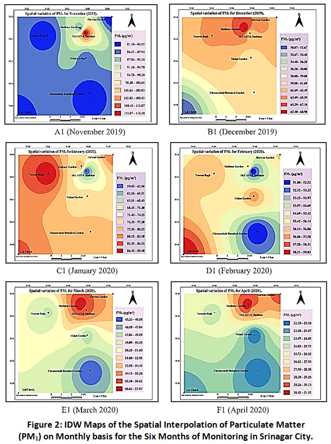Figure 2: IDW Maps of the Spatial Interpolation of Particulate Matter (PM1) on a Monthly basis for the Six Months of Monitoring in Srinagar City. Click here to view Figure

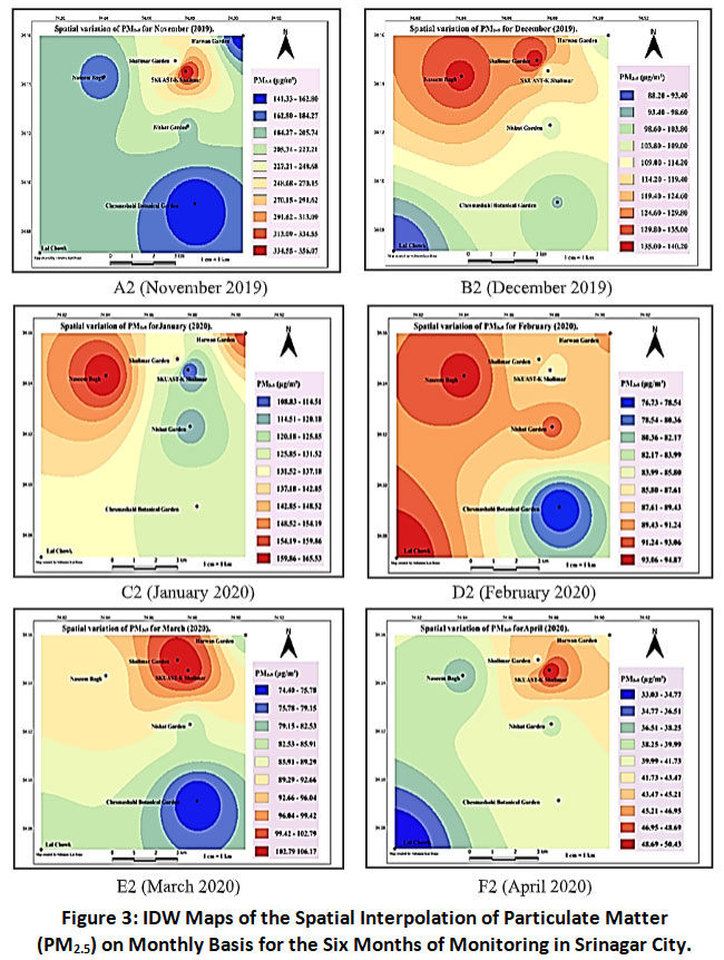Figure 3: IDW Maps of the Spatial Interpolation of Particulate Matter (PM2.5) on Monthly Basis for the Six Months of Monitoring in Srinagar City. Click here to view Figure

Figure 4: IDW Maps of the Spatial Interpolation of Particulate Matter (PM4) on Monthly Basis for the Six Months of Monitoring in Srinagar City. Click here to view Figure

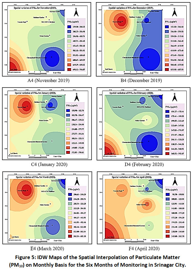Figure 5: IDW Maps of the Spatial Interpolation of Particulate Matter (PM10) on Monthly Basis for the Six Months of Monitoring in Srinagar City. Click here to view Figure

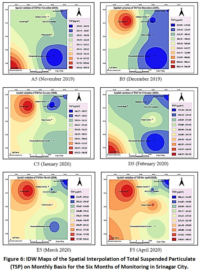Figure 6: IDW Maps of the Spatial Interpolation of Total Suspended Particulate (TSP) on Monthly Basis for the Six Months of Monitoring in Srinagar City. Click here to view Figure

Figure 7: IDW Maps of the Spatial Interpolation of Carbon Dioxide (CO2) on Monthly Basis for the Six Months of Monitoring in Srinagar City. Click here to view Figure

Table 2: Average Daytime Concentrations of Pollutants at the Monitoring Sites for the Six Months of Sampling. Click here to view Table

Table 3: Six-Month Average Concentration of Particulate Matter (μg/m³) and Carbon Dioxide (ppm) at Each Monitoring Site in Srinagar City.

Critical Difference (CD) is significant at p ≤ 0.05; SE(d) is the standard error of the difference.

Table 4: Pearson Correlation Matrix of Particulate Matter Carbon Dioxide based on the Monthly Average for all Locations.

* Significant at p ≤ 0.05;

** Significant at p ≤ 0.01.

The average daytime (morning, afternoon, and evening) concentrations of the monitored pollutants for the monitoring sites are depicted in Table 2. From the data, it can be observed that for each monitored pollutant at most of the monitoring sites and the average mean daytime concentrations of pollutants, the morning and evening concentrations were highest. For example, the average mean daytime concentration of PM₁ was highest in the morning (67.07 µg/m³) followed by the evening (57.62 µg/m³) and then the afternoon. The same trend was followed by PM_{2.5 ­} and PM₄. But, with the larger particles (PM₁₀ and TSP) and CO_2, the average mean daytime concentration was highest in the evening followed by the morning and then the afternoon. This can be attributed to a lot of vehicular movements in the morning as people drive to their different working places and in the evening as they drive from the same. Also, traffic congestion in Srinagar city is observed mainly in the morning and the evening times of the day. During the winter months (November – January), the high biomass burning for heating purposes that are observed around the various monitoring sites plus the lesser atmospheric wind to disperse particles and CO₂, and the high level of humidity keeps particles particularly the larger ones stagnated in the ambient air for long period especially in the morning and evening. It has been proven by many research data that pollutants transport from a long-range, lower atmospheric mixing, and less dispersion of pollutants, especially during the winter are responsible for higher pollution as pollutants are always stagnant in the lower atmosphere^15,32,33.

The data (Table 3) shows the six months average variation of the pollutants monitored in this investigation from November 2019 to April 2020 at the different sampling sites/locations. The data shows that for all/most of the pollutants monitored, Chesmashahi Botanical Garden and Harwan Garden exhibited the least concentrations respectively. This can be attributed to the fact that both tourists’ sites are located at more serene locations experiencing less vehicular movement and traffic. Also, there are a smaller number of residential houses around these tourists’ sites especially Chesmashahi Botanical Garden, and therefore not much affected by burning during the winter season. The six-month average concentration of the smaller particles (PM ≤ 4 μm) was recorded highest at Shalimar Garden (63.61 μg/m³ for PM₁) and SKUAST-K Shalimar (136.89 and 169.65 μg/m³ for PM_2.5 and PM₄ respectively). Whereas, the larger particles (PM₁₀ and TSP) were recorded highest at Naseem Bagh (430.87 and 578.38 μg/m³) and Lal Chowk (420.57 and 528.42 μg/m³) respectively. The highest level of CO₂ was recorded at Shalimar Garden (610.56 ppm). Due to the high traffic, the high concentration of houses, and biomass burning around these sites might have enhanced their pollutants concentrations. Areas that often have high traffic have been considered as hotspots for suspended particulate matter.³⁰ The average six months spatial variation of the concentration of the monitored pollutants was statistically significant (p ≤ 0.05) between most of the monitoring sites. The correlation of particulate matter and CO₂ given in Table 4 shows a positive correlation even though non-significant between the monthly concentration of most pollutants. Nevertheless, PM₁, PM_2.5, and PM₄ show a significant (p ≤ 0.01) strong positive correlation with each other. Also, PM₄ and PM₁₀, and likewise PM₁₀ and TSP had a significant (p ≤ 0.05) strong positive correlation with each other. The positive correlation shows how the increase of any of these parameters will cause a corresponding increase of the other. Particulate matter concentration has been found to have a mutual correlation with outdoor/ambient environment.³¹

Conclusion

From the data and IDW maps obtained, it was clear that there was a significant monthly spatial variation of the concentration of all the monitored pollutants between most of the monitoring sites and their surrounding unsampled areas. Also, the spatial variation of the average six months concentration of monitored pollutants was statistically significant (p ≤ 0.05) between most of the monitoring sites. This might be attributed to the location of the monitoring sites, changes in traffic flow, different seasonal (winter and spring) activities like biomass burning, and weather conditions like atmospheric temperature, wind speed, precipitation, and relative humidity. This informs us that the concentration of particulate matter and carbon dioxide varies on monthly basis with distance from one location to another in Srinagar city. Also, the data proves that the ambient air in Srinagar city experiences increasing pollution in the morning and evening than in the afternoon. And that all the parameters/pollutants correlate positively with each other, that is, they all increase with each other simultaneously even though most are insignificantly positively correlated. The sources of pollution with their estimated source proportion in the city have been noted by the Jammu and Kashmir State Pollution Control Board in a report on managing air quality in Srinagar city as follows: vehicular emission (65-75 %), dust from bad roads (10-15 %), biomass and garbage burning (10-20 %), construction and demolition emissions (5-8 %), minor industrial activities (7-8 %) and other sources (3 %).⁶ Thus causing the deteriorating condition of the city’s ambient air. It is therefore concluded that the poor air quality of Srinagar city varies with distance as depicted by the data and IDW maps with respect to the monitoring sites and the monitored pollutants. Thus, giving an idea of the pollutants blanket over the city. In the future, a more expanded study with regards to this work is recommended to be carried out covering the whole Srinagar district.

Acknowledgment

For the completion of this work, the administration of the Division of Environmental Sciences, Sher-e-Kashmir University of Agricultural Sciences and Technology, Shalimar campus is appreciated for the necessary support given in this research.

Funding Sources

No funding was received for the research, authorship, and/or publication of this article.

Conflict of Interest

The author(s) declares no conflict of interest.

References

1. Institute, Health Effect. State of Global Air 2018. Special Report.; 2018. https://www.stateofglobalair.org/sites/default/files/soga-2018-report.pdf.
2. Lee KK, Miller MR, Shah ASV. Air pollution and stroke. J Stroke. 2018;20(1). doi:10.5853/jos.2017.02894.
   CrossRef
3. WHO. Ambient (outdoor) air pollution. Published 2018. Accessed April 10, 2021. https://www.who.int/news-room/fact-sheets/detail/ambient-(outdoor)-air-quality-and-health.
4. Kulshrestha UC. PM₁ is More Important than PM2.5 for Human Health Protection. Curr World Environ. 2018;13(1). doi:10.12944/cwe.13.1.01.
   CrossRef
5. Hedley C, Saggar S, Tate K. Procedure for fast simultaneous analysis of the greenhouse gases: Methane, carbon dioxide, and nitrous oxide in air samples. Commun Soil Sci Plant Anal. 2006;37(11-12). doi:10.1080/00103620600709928.
   CrossRef
6. Anonymous. Revised Action Plan for Air Quality Management in Srinagar city. In: Revised Action Plan Control of Air Pollution in Non-Attainment Cities Jammu and Srinagar. ; 2018:28-44. http://jkspcb.nic.in/WriteReadData/userfiles/file/Ambient Air Quality/Action Plan on Control of Air Pollution in Non-Attainment Cities.pdf.
7. Nikhil ST. Study on the effect of vehicular pollution on the ambient concentrations of particulate matter and carbon dioxide in Srinagar city. Published online 2020. DOI: Available in SKUAST-K Library, Shalimar.
8. Nusret D, Dug S. Applying the Inverse Distance Weighting and Kriging methods of the spatial interpolation on the mapping the annual precipitation in Bosnia and Herzegovina. In: IEMSs 2012 - Managing Resources of a Limited Planet: Proceedings of the 6th Biennial Meeting of the International Environmental Modelling and Software Society.; 2012.
9. Fontes T, Barros N. Interpolation of air quality monitoring data in an urban sensitive area: the Oporto/Asprela case. Edições Univ Fernando Pessoa. 2010;7:6-18. https://bdigital.ufp.pt/handle/10284/2334.
10. Kumar Jha D, Sabesan M, Das A, Vinithkumar N V, Kirubagaran R. Evaluation of Interpolation Technique for Air Quality Parameters in Port Blair, India. Univers J Environ Res Technol. 2011;1(3).
11. Li L, Losser T, Yorke C, Piltner R. Fast inverse distance weighting-based spatiotemporal interpolation: A web-based application of interpolating daily fine particulate matter PM2:5in the contiguous U.S. using parallel programming and k-d tree. Int J Environ Res Public Health. 2014;11(9). doi:10.3390/ijerph110909101.
    CrossRef
12. Kumar A, Krishna A. Aerosol concentration over Ranchi urban area and South Karanpura Coalfield region, Jharkhand, India-A comparative geospatial appraisal. J Ind Geophys Union. 2017;21(5):431-440.
13. Schloeder CA, Zimmerman NE, Jacobs MJ. Comparison of Methods for Interpolating Soil Properties Using Limited Data. Soil Sci Soc Am J. 2001;65(2). doi:10.2136/sssaj2001.652470x.
    CrossRef
14. Arumugam T, Kunhikannan S, Radhakrishnan P. Assessment of fluoride hazard in groundwater of Palghat District, Kerala: A GIS approach. Int J Environ Pollut. 2019;66(1-3). doi:10.1504/IJEP.2019.104533.
    CrossRef
15. Hakim ZQ, Beig G, Reka S, Romshoo SA, Rashid I. Winter Burst of Pristine Kashmir Valley Air. Sci Rep. 2018;8(1). doi:10.1038/s41598-018-20601-z.
    CrossRef
16. Met One Instruments. Fine Dust Meter Met One AEROCET 831. Website. DOI: AEROCET 831.
17. Met One Instruments. Comet Software. Website. Published 2019. Accessed October 24, 2019. https://metone.com/products/comet/
18. Remer LA, Kaufman YJ, Tanré D, et al. The MODIS aerosol algorithm, products, and validation. J Atmos Sci. 2005;62(4). doi:10.1175/JAS3385.1.
    CrossRef
19. Baschant D, Stahl H. Temperature resistant IR-gas sensor for CO2 and H2O. In: Proceedings of IEEE Sensors. Vol 1. ; 2004.
20. Hodgkinson J, Smith R, Ho WO, Saffell JR, Tatam RP. Non-dispersive infra-red (NDIR) measurement of carbon dioxide at 4.2 μm in a compact and optically efficient sensor. Sensors Actuators, B Chem. 2013;186. doi:10.1016/j.snb.2013.06.006.
    CrossRef
21. Rave Innovations. Realtime Portable CO₂ Monitor- CDM 901. Website. Published 2019. Accessed October 25, 2019. http://www.erave.in/products/index.html.
22. Lu GY, Wong DW. An adaptive inverse-distance weighting spatial interpolation technique. Comput Geosci. 2008;34(9). doi:10.1016/j.cageo.2007.07.010.
    CrossRef
23. McCoy J, Johnston K, Kopp, Borup B, Willison J, Payne P. ArcGIS 9. 1st ed. ESRI; 2001.
24. Salih IM, Pettersson HBL, Sivertun A, Lund E. Spatial correlation between radon (222-Rn) in groundwater and bedrock uranium (238-U): GIS and geostatistical analyses. J Spat Hydrol. 2002;2(2).
25. Sheikh M, Najar IA. Preliminary Study on Air Quality of Srinagar, (J&K), India. J Environ Sci Stud. 2018;1(1). doi:10.20849/jess.v1i1.421.
    CrossRef
26. Lau J, Hung WT, Cheung CS. Interpretation of air quality in relation to monitoring station’s surroundings. Atmos Environ. 2009;43(4). doi:10.1016/j.atmosenv.2008.11.008.
    CrossRef
27. Li A, Chen C, Chen J, Lei P. Environmental investigation of pollutants in coal mine operation and waste dump area monitored in Ordos Region, China. RSC Adv. 2021;11(17). doi:10.1039/d0ra10586d.
    CrossRef
28. Awasthi A, Agarwal R, Mittal SK, Singh N, Singh K, Gupta PK. Study of size and mass distribution of particulate matter due to crop residue burning with seasonal variation in rural area of Punjab, India. J Environ Monit. 2011;13(4). doi:10.1039/c1em10019j.
    CrossRef
29. Jayamurugan R, Kumaravel B, Palanivelraja S, Chockalingam MP. Influence of Temperature, Relative Humidity and Seasonal Variability on Ambient Air Quality in a Coastal Urban Area. Int J Atmos Sci. 2013;2013. doi:10.1155/2013/264046.
    CrossRef
30. Kale US, Sawant P. Evaluation of Impact of Particulate Matter on Traffic Personnel and at Traffic Junctions. J Environ Heal Sci. 2016;2(6):1-9. doi:10.15436/2378-6841.16.1037.
    CrossRef
31. Pan S, Du S, Wang X, et al. Analysis and interpretation of the particulate matter (PM₁₀ and PM_2.5) concentrations at the subway stations in Beijing, China. Sustain Cities Soc. 2019;45. doi:10.1016/j.scs.2018.11.020.
    CrossRef
32. Tiwari S, Chate DM, Srivastava MK, et al. Statistical evaluation of PM₁₀ and distribution of PM₁, PM_2.5, and PM₁₀ in ambient air due to extreme fireworks episodes (Deepawali festivals) in megacity Delhi. Nat Hazards. 2012;61(2). doi:10.1007/s11069-011-9931-4.
    CrossRef
33. Chakraborty T, Beig G, Dentener FJ, Wild O. Atmospheric transport of ozone between Southern and Eastern Asia. Sci Total Environ. 2015;523. doi:10.1016/j.scitotenv.2015.03.066.
    CrossRef