A Comprehensive Assessment of Land Use Land Cover of Thiruvananthapuram Urban Agglomeration using GIS and Remote Sensing
R S Anupriya
*
 and T A Rubeena
1
Department of Geography,
University College,
Thiruvananthapuram,
Kerala
India
http://dx.doi.org/10.12944/CWE.17.3.19
Copy the following to cite this article:
Anupriya R. S, Rubeena T. A. A Comprehensive Assessment of Land Use Land Cover of Thiruvananthapuram Urban Agglomeration using GIS and Remote Sensing. Curr World Environ 2022;17(3). DOI:http://dx.doi.org/10.12944/CWE.17.3.19
Copy the following to cite this URL:
Anupriya R. S, Rubeena T. A. A Comprehensive Assessment of Land Use Land Cover of Thiruvananthapuram Urban Agglomeration using GIS and Remote Sensing. Curr World Environ 2022;17(3).
Download article (pdf)
Citation Manager
Publish History

Introduction
The quick and dramatic rise in population of South East Asian countries especially in India, has occurred over the last century accentuated the demand for basic needs1. Hence it has become pertinent to rationally utilize the available land and other resources. Currently a drastic change in Land use/ Land cover is observed2,3. The term ‘Land use’(LU) denotes how land is utilized by humans, while ‘land cover’(LC) refers to natural features that cover the land4. The rapid and uncontrolled momentum of urbanization is a leading element behind the drastic land use changes. The process of urbanization has significant implications upon the physical, socio-cultural, economic and demographic aspects of a landscape. Although being considered as a positive factor of development, urbanization poses some serious threats to the natural environment. The unplanned and unscientific urbanization forces negatively impact various components of the urban niche such as its micro climate, groundwater resources potential, land cover pattern, hazardous mitigation and food and security policies5-,9. The urban scenario of the world is undergoing a radical revolution as it progresses with industrialization and modernization. Rampant urbanization has been taking place due to various factors such as natural increase of population and probably due to movement of people from adjoining countryside to the city for improved employment prospects and enhanced standard of living, rapid economic development and associated infrastructure development5,10,11. According to the UN report, the share of world population lived in urban centres in 1950’s was 30%. The trend has gone up ever since, with 55% of world population living in urban areas in 2018 and is projected to be 68% in the year 2050 where the highest rate of increase will be recorded in developing nations12.
Like any other developing country, urbanization in India has also risen in an exponential manner in the last few decades13,14. In India, the trend of urbanization shows a rapid increase from 27.7% to 31.1% with a growth rate of 3.3% during 2001–2011 as compared to the rate of 2.1% increase during 1991–200115. Further, the studies show that, India will account nearly 600 million urban population by 203116 and eventually will host 814 million in 2050, which will become the highest urban population in the world14. As per 2011 census, high level of urbanization has been reported in Kerala as against low population growth rates6. Apart from the other parts of the country, Kerala presents a unique picture of urban- rural continuum spreading across the entire state with an exception of some hilly tracks of upland region of the state. The urban share of the state as per 2011 census is 47.78 percent17. To accommodate such increasing urban population, cities expand their spatial limits beyond the political boundary, which will exert immense pressure on surrounding natural landscapes often leads to LU/ LC change5,14. Geographic understanding of LU/ LC change is a key source of urban related impact analysis. For achieving the goals of sustainable urban development, availability of changes in land use statistics is essential for decision-making process18. Therefore, a thorough understanding of undercurrents of urbanization induced land cover change is essential for coping with environmental changes5.
Geospatial tools such as remote sensing and GIS has emerged as powerful techniques in the field of land resources evaluation and management4. There are several studies that have attempted to evaluate extend of land use changes using geospatial techniques19- 25. Considering the significance of these changes in fast-growing cities and towns and for making the developments eco-friendlier, the main aim of the research is to estimate the magnitude of LU/ LC changes and its dynamics in Thiruvananthapuram city and fringe area during the period 1988–2018.
Study area
Thiruvananthapuram also known as Trivandrum, the administrative headquarters of the South Indian state Kerala, is a rapidly growing urban agglomeration. With a population of 957,730 Thiruvananthapuram forms the most populous city in Kerala as of 201117 census. Being the largest city down South, Thiruvananthapuram has an urban agglomeration population of around 1.68 million and forms the biggest Information Technology (IT) hub with 55% of the state's software exports26. Being in the humid tropics, the region experiences monsoon dominated tropical climate with two distinct seasons. Physiographically, the region is sandwiched between the mighty Western Ghats in the East and Arabian Sea in the West (Figure 1). Being located near the international ocean route and the presence of inland water ways and road connectivity, Thiruvananthapuram forms an ideal location for rapid urban development.
To study the land use/ land cover changes and urban dynamics in Thiruvananthapuram and adjoining areas, a 5 km buffer zone around Thiruvananthapuram Municipal Corporation (TMC) is created and the panchayats falling under the aforesaid 5 km buffer is selected for the present study (Figure1).
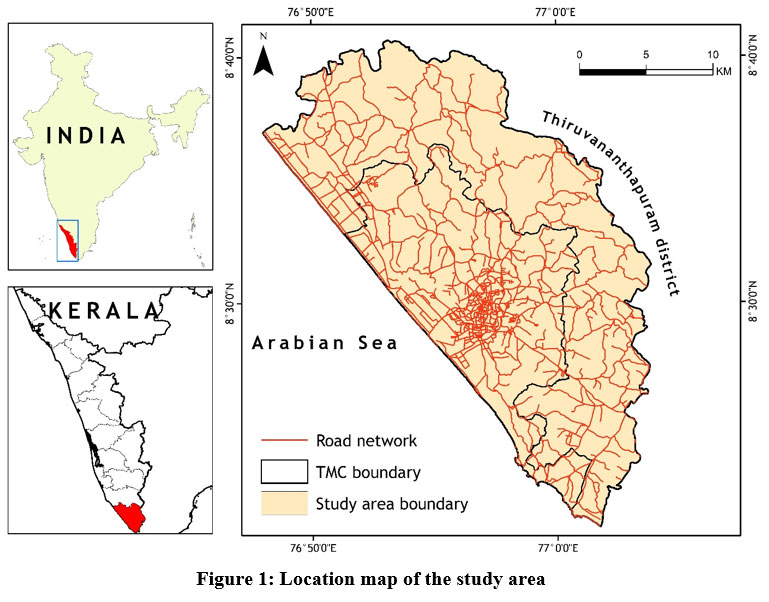 | Figure 1: Location map of the study area.
|
The TMC together with selected panchayats forms the study areas with an aerial extend of 527.96km2 and a total population of 1562943.
Materials and Method
A GIS and remote sensing based comprehensive methodology comprising of six major phases was adopted for the study. The methodology flow chart is given in Figure.2 and it consists of (1) data collection procedures, (2) pre-processing steps, (3) selection of training sites, (4) image classification, (5) accuracy assessment, and (6) assessment of LU/LC changes over time.
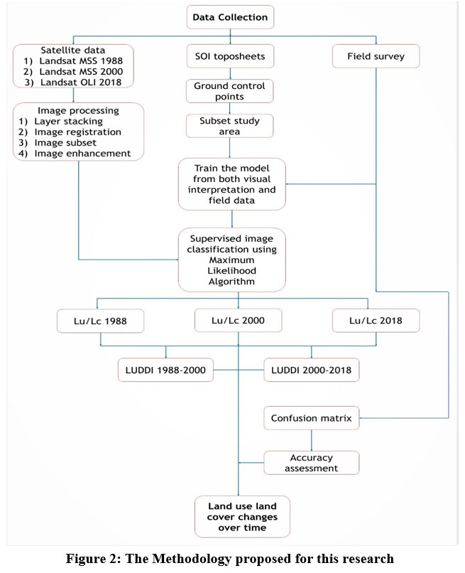 | Figure 2: The Methodology proposed for this research.
|
As the first step, the TMC boundary is collected from Municipal Corporation office and the boundaries of adjoining panchayats were gathered from Kerala State Remote Sensing and Environment Centre (KSREC). Thereafter with the help of SOI topographical sheets (Scale 1:50000) the positional accuracy is cross checked and boundary map is prepared (Figure 1). The next step was the selection of satellite images for the classification.
Landsat series of mission 5 TM (Thematic Mapper), mission 7 ETM+ (Enhanced Thematic Mapper Plus) and mission 8 OLI (Operational Land Imager) were selected for the path and row of 144 and 54 were utilized11. The images acquired on the dates of 19/01/1988, 27/11/2000 and 08/01/2018 respectively. All the imageries used here had spatial resolution of 30 meter11, 27 and were obtained by the satellites during day time and were chosen based on the availability of cloud free data. Both imageries of 1988 and 2018 were characterized with least cloud cover of one percent and the image of 2000 was characterized with two percent of cloudiness, which is less than the advisable cloud cover (<10%)27 for LU/LC studies.
The quality of the images was enhanced through pre-processing techniques in ERDAS Imagine 9.3. The SOI topographical sheets were used as a reference to reduce geometric distortions and image enhancement techniques such as histogram equalization is used to improve spectral responses. All the sub set images were given a common coordinate system of UTM_WGS_1984 43N zone.
The present study has utilized Maximum Likelihood (MLC) method to classify the selected satellite images. MLC has been proven as an efficient classification algorithm in medium resolution images28,29. For the classification purpose the spectral signatures were developed through visual interpretation techniques. According to Hexagon geospatial, MLC computes the weighted distance ‘DW ’of an unknown vector ‘X’ belonging to one of the known classes “i” is based on the Bayesian equation29,30:
.jpg)
Where ‘c’ indicates a particular class, ‘ai’ denote probability of a pixel which is a part of class ‘i’. In order to remove speckle noises in the image,4x4 kernels were used after classifying the data30,31.
To understand land use dynamism of the study area, Land use Dynamic Degree Index (LUDDI) by Han was employed32. LUDDI represent proportional variation in LU/LC categories for a selected time period. This index reflects spatio-temporal changes of LU/LC patterns.
The LUDDI is determined by:
.jpg)
Whereas is the area of land use type ‘i’ in the beginning of the period, is the total area of a land use type ‘i’ converted into other types and ‘t’ is the study period. The classified satellite images were cross-checked to ensure its classification accuracy. For this a total of 278 points for 1988, 2000 and 2018 were generated from field survey and random point’s generation through visual image interpretation. Two error matrices were created for 1988-2000 period and 2000-2018 period and from these two matrices, both classification error and classification accuracy were computed. The errors in image classification are omission and commission error. Commission error can be defined as the error which occurs when a classification process assigns pixels to a specific class that does not belong to it. The omission error occurs when pixels that belong to one class, are included in other classes. The post classification accuracy was checked using confusion matrix-based methods such as Producer’s accuracy, user’s accuracy, overall accuracy, and Kohen’s Kappa index (K) which can be estimated using equation 3 to 6 respectively14.
.jpg)
Where, ‘N’ stands for total pixel numbers, ’r’ indicate number of classes,’xkk’ connotes all pixels in the ‘k’ column and ‘k’,xk+ refer to total samples in ‘k’ row, and ‘x+k’ on the error matrix for total samples in ‘k’.
Results and Discussion
Land use/land cover change (LU/LC)
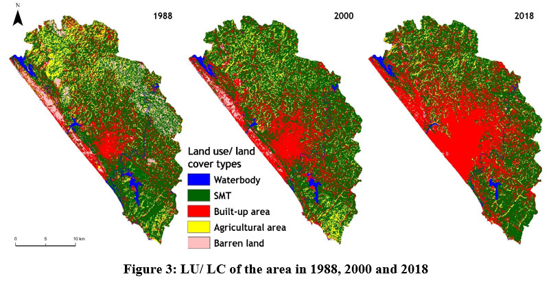
Figure 3 shows changes in LU/LC in the study area during 1988, 2000 and 2018.The generalized land use/ land cover categories following NRSC (National Remote Sensing Centre) classification scheme such as water body, settlements with mixed trees (hence forth referred to as SMT), built-up land, agricultural area and barren land were identified. Settlement with mixed trees is a unique land use/ land cover class identified here, due to presence of canopy covered urban- rural continuum. In this category, settlement area is intricately mixed with natural vegetation and therefore is it is impractical to separate both, while using imageries of 30m spatial resolution. Hence this class has the characteristics of both settlements and vegetation.
 | Figure 3: LU/ LC of the area in 1988, 2000 and 2018
|
In the year 1988, SMT was the dominant Land use/Land cover covering 56.92 % (Table 1). Built-up area, agricultural area, barren land, and water bodies constituted 19.34%, 14.11%, 7.01% and 2.63% respectively. In 2000, the SMT class slightly increased to 58.40%. However, water body (2%), barren land (2.36%) and agricultural area (10.35%) show a decreasing trend. In contrast built-up area shows a steady increase from 19.35% in 1988 to 26.88% in 2000.
Table 1: LULC Changes From 1988 To 2000
| 1988 | 2000 | 2018 | |||
Land use/ Land cover types | Area (in km2) | Area % | Area (in km2) | Area % | Area (in km2) | Area % |
Water body (WB) | 13.88 | 2.63 | 10.57 | 2.00 | 8.42 | 1.60 |
Built-up area (BT) | 102.08 | 19.34 | 141.93 | 26.88 | 220.33 | 41.73 |
Settlements with Mixed Trees (MT) | 300.50 | 56.92 | 308.35 | 58.40 | 256.36 | 48.56 |
Agricultural area (AG) | 74.51 | 14.11 | 54.65 | 10.35 | 38.01 | 7.20 |
Barren land (BL) | 36.99 | 7.01 | 12.45 | 2.36 | 4.83 | 0.91 |
Total | 527.95 | 100% | 527.95 | 100% | 527.95 | 100% |
Accuracy Assessment
Accuracy assessment was performed in LU/LC map of 1988, 2000 and 2018 and the results are furnished in tables 3, 4 and 5. For 1988 map, a total of 96 random pixels are generated and analyzed using error matrix. The 1988 map has an overall classification accuracy of 0.865 or 86.5% and K coefficient of 0.885 (table 3). In 1988 map Water body shows highest producer’s accuracy of 100% with least omission error of 0.00. However, SMT class shows lowest producers’ accuracy of 68.75 (Table 2). In the case of user’s accuracy, four classes (barren land, water body, built-up area, and agricultural area) show accuracy above 80%, whereas SMT shows lowest user’s accuracy of 78.57%. In the case of commission error also barren land shows least error (0.050) whereas built-up area shows maximum error (0.214).
Table 2: Accuracy Assessment of LULC Classification of 1988 Using Error Matrix
LU/LC | WB | AG | BT | SMT | BL | Total | Error: Commi | User's |
WB | 17 | 0 | 1 | 0 | 0 | 18 | 0.056 | 94.44 |
AG | 0 | 20 | 0 | 5 | 0 | 25 | 0.200 | 80.00 |
BT | 0 | 0 | 16 | 0 | 3 | 19 | 0.158 | 84.21 |
SMT | 0 | 3 | 0 | 11 | 0 | 14 | 0.214 | 78.57 |
BL | 0 | 0 | 1 | 0 | 19 | 20 | 0.050 | 95.00 |
Total | 17 | 23 | 18 | 16 | 22 | 96 | Overall accuracy 0.865 Kappa 0.885 | |
Error: Ommi | 0.000 | 0.130 | 0.111 | 0.313 | 0.136 |
| ||
Producer’s | 100.00 | 86.96 | 88.89 | 68.75 | 86.36 |
| ||
Table 3: Accuracy Assessment of LULC Classification of 2000 Using Error Matrix
LU/LC | WB | AG | BT | SMT | BL | Total | Error: Commi | User's accu |
WB | 13 | 0 | 1 | 0 | 0 | 14 | 0.087 | 91.30 |
AG | 0 | 10 | 0 | 3 | 0 | 13 | 0.214 | 78.57 |
BT | 0 | 0 | 34 | 5 | 2 | 41 | 0.059 | 94.12 |
SMT | 0 | 2 | 0 | 15 | 0 | 17 | 0.040 | 95.65 |
BL | 0 | 0 | 2 | 0 | 4 | 6 | 0.250 | 75.00 |
Total | 13 | 12 | 37 | 23 | 6 | 91 | Overall accuracy 0.879 Kappa 0.863 | |
Error: Ommi | 0.045 | 0.043 | 0.238 | 0.185 | 0.000 |
| ||
Producer’s accu | 95.45 | 95.65 | 76.19 | 81.48 | 100.00 |
| ||
For the 2000 map, 91 pixels were chosen randomly and the overall accuracy reported is 0.879 or 87.9% percentage with a Kappa coefficient of 0.863 (Table 3). In 2000, three LU/LC classes like SMT, built- up area and waterbody reported User’s accuracy above 90% (i.e., 95.65%, 94.12% and 91.30% respectively) while both agricultural area and barren land reported 78.57% and 75% accuracy respectively. Subsequently, lowest commission error is noticed in SMT (0.040) and highest commission error in barren land (0.250). The creator’s accurateness for each class is greater than 75%. However, maximum producer’s accuracy is reported for barren land and least for built-up area (Table 4). It is also noted that the error of omission is 0.00 in barren land.
Table 4: Accuracy Assessment of LULC Classification of 2018 Using Error Matrix
LU/LC | WB | AG | BT | SMT | BL | Total | Error: Commi | User's |
WB | 13 | 0 | 1 | 0 | 0 | 14 | 0.071 | 92.86 |
AG | 0 | 10 | 0 | 3 | 0 | 13 | 0.231 | 76.92 |
BT | 0 | 0 | 39 | 0 | 2 | 41 | 0.049 | 95.12 |
SMT | 0 | 2 | 0 | 15 | 0 | 17 | 0.120 | 88.24 |
BL | 0 | 0 | 2 | 0 | 4 | 6 | 0.330 | 66.67 |
Total | 13 | 12 | 42 | 18 | 6 | 91 | Overall accuracy 0.890 Kappa 0.837 | |
Error: Ommi | 0.000 | 0.167 | 0.071 | 0.167 | 0.333 |
| ||
Producer’s | 100.00 | 83.33 | 92.86 | 83.33 | 66.67 |
| ||
WB waterbody, AG agricultural area, BT built-up area, and BL Barren land.
The LU/LC map of 2018 reported highest overall accuracy of 89% which indicates that fine spectral resolution of Landsat 8 OLI image has better ability to differentiate the earth surface features in medium resolution compared to Landsat 5 MSS. For 2018 LU/LC map, the user’s accuracy varies from 95.12 (built-up area) to 66.67% (barren land). Subsequently, the minimum commission error is also reported in built-up area class (0.049) (Table 4). In the case of producer’s accuracy, water body reported 100% accuracy and zero omission error whereas barren land shows minimum producer’s accuracy (66.67%) with maximum omission error (0.033). The reported Kappa coefficient of 2018 LU/LC map is 0.837, which indicates sufficient accuracy of the classification. In general, all the three LU/LC maps have overall accuracy above 85% and Kappa coefficient above 0.8, which indicates higher accuracy of the classified images. Therefore, these LU/LC maps were further processed for land use conversion analysis.
Urban Sprawl and Land Use/Land Cover Conversion
Throughout the twelve-year duration from 1988 to 2000, considerable land use conversion has taken place in the study area. For instance, agricultural area shows a remarkable decrease from 74.51km2 in 1998 to 54.65 km2 in 2000. A significant portion of the agricultural area is converted into SMT and built-up area. Nearly 52.30% of this agricultural area was converted into SMT, which can be attributed to the recent land reclamation trend in Kerala, where many of agricultural lands were reclaimed and converted to settlements and small-scale plantation areas. Another important land use type that witnessed major conversion is the barren land. During 1988, the percentage of barren land in the study area was 7.01% which declined to 2.36% in 2000. It is noticed that 38.42% of barren land is converted into SMT and 34.90% is converted into built-up areas suggesting the process of urbanisation gradually transforming the fringe landscape (table 5). It is also observed that only 2.30% is converted to agricultural area, which indicates that the new agricultural initiatives were reducing and cropping pattern is slowly changing from traditional crops to plantation-oriented crops in the study area. However, the areal extension of SMT shows a slight increase from 1988 to 2000. Even though a significant amount of SMT is converted into built-up area, it is outweighed by agricultural to SMT conversion. During the 1988-2000 period, the area under water body has reduced from 2.60% to 2% and the difference of 0.6% is negligible.
Table 5: LU/ LC Change Matrix of 1988-2000 (In Percentage).
LU/LC | Water body | Built-up area | SMT | Agricultural area | barren land | 1988 Total |
Waterbody | 9.28 | 2.85 | 1.43 | 0.21 | 0.10 | 13.88 |
Built-up area | 0.58 | 61.48 | 34.37 | 3.47 | 2.19 | 102.08 |
SMT | 0.39 | 54.91 | 219.37 | 24.97 | 0.87 | 300.50 |
Agricultural area | 0.11 | 9.78 | 38.97 | 25.16 | 0.48 | 74.51 |
barren land | 0.21 | 12.91 | 14.21 | 0.85 | 8.81 | 36.99 |
2000 Total | 10.57 | 141.93 | 308.35 | 54.65 | 12.45 | 527.95 |
The rate of urban sprawl and related land use/ land cover changes is more rapid in the second phase of the study (i.e., from 2000 to 2018) than the first phase (1988 to 2000). The study reveals an increase of 22.40% in built-up area during 1988-2018 (Figure 4a), whereas it was only 7.54% in the first phase (i.e., 1988 to 2000) (table 5). The developmental activities including construction of residential, commercial buildings and non-commercial units and basic infrastructures such as road network increased dramatically in the region. Urban sprawl in the area exhibits a close relationship with road networks as well as outward shift from the city center (Figure 4a). The presence of road network is the most significant driver of urban sprawl as it provides access to major hotspots and other facilities33. The decline of SMT is shown in Figure 4b. It is noticed that during the first phase (1988-2000), the areal extent of SMT increased from 56.92% to 58.40% (+1.48%). However, it has declined by about 9.85% during the 2000-2018 period and 30.46% of the SMT area were converted into built-up area by 2018. Since SMT is having both settlements and vegetation, the slight increase can be associated with rural built-up development that occurred during 1988-2000 phase. However, in the second phase, the rate of urban growth outweighs rural settlement developments and the study area shows a city centre focused growth than a decentralized one (Figure 4a and 4b). It is also observed that in the second phase, except built-up area all other land use classes show a decreasing trend, which is the result of rapid urban growth in the study area (Table 6). Arulbalaji11 also reported the rapid urbanization in cities similar to Thiruvananthapuram. In the second phase also the conversion of agricultural area remains high with approximately 61.65% of the agricultural areas getting converted to SMT type which is the result of both land reclamation and greater preference for plantation-oriented crops. However, a significant amount of agricultural area is converted to built-up area (table 6). During the 18-year interval of 2000-2018 period, ~72.21% of barren land is converted into built-up area (Table 6). The drastic change of barren land is also visible in Figure 3. Unlike the first phase, the second phase witnessed a drastic decline of water bodies in the study area from 2% in 2000 to 1.6% in 2018. The major decline is witnessed in lakes than rivers, for instance Akkulam Lake shows a high rate of areal shrinkage from 1988 to 2018. The decline of water bodies, due to urbanization in Thiruvananthapuram is also reported by previous authors6,10.
Table 6: LU/ LC Change Matrix of 2000-2018 (In Percentage).
LU/LC | Water body | Built-up area | SMT | Agricultural area | Barren Land | 2000 Total |
Waterbody | 7.22 | 1.23 | 1.36 | 0.48 | 0.27 | 10.57 |
Built-up area | 0.65 | 108.46 | 25.33 | 6.23 | 1.27 | 141.93 |
SMT | 0.43 | 93.91 | 195.19 | 18.02 | 0.80 | 308.35 |
Agricultural area | 0.05 | 7.74 | 33.69 | 13.01 | 0.16 | 54.65 |
barren land | 0.07 | 8.99 | 0.80 | 0.27 | 2.32 | 12.45 |
2018 Total | 8.42 | 220.33 | 256.36 | 38.01 | 4.83 | 527.95 |
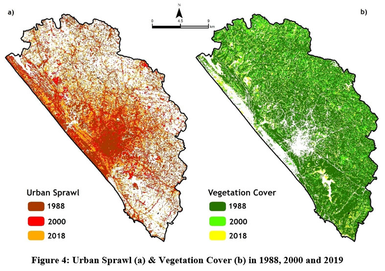 | Figure 4: Urban Sprawl (a) and Vegetation Cover (b) in 1988, 2000 and 2019.
|
LUDDI from 1988 to 2018.
The degree of land use dynamics is calculated with LUDDI and presented in Table 7. During both the phases (i.e., 1988-2000 and 2000-2018) significant land use changes have occurred. Cumulative LUDDI of 1988-2000 is higher than the 2000-2018 phases. For the sake of assessing the spatial variability in land use dynamics, both 1988-2000 and 2000-2018 phases are mapped and are depicted in Figure 5a and Figure 5b.
Table 7: LUDDI from 1988 to 2018
LU/LC | LUDDI of 1988-2000 | LUDDI of 2000-2010 |
Waterbody | 2.76 | 1.76 |
Built-up area | 3.27 | 1.31 |
SMT | 2.25 | 2.04 |
Agricultural area | 5.52 | 4.23 |
Barren land | 6.35 | 4.52 |
Cumulative LUDDI | 20.15 | 13.86 |
From the LUDDI it is noted that both agricultural area and barren land reported highest LUDDI values and remains the most dynamic land use class during both the phases (i.e., 1988-2000 and 2000-2018) (Table 8). The dynamic nature of both the classes are the outcome of swift urbanization and related land use shifts. An unscientific and utmost level of the land use conversion and land reclamation processes are turn out in Kerala. As a result, agricultural areas including paddy fields and wetlands are reclaimed for basic infrastructure development and built-up area development. In Figure 5, it can be seen that LUDDI of barren land is classified as high in both phases. It is also visible that barren lands along the western coastal edges of the city are rapidly getting converted into built-up areas. This was primarily due to the outgrowth of Kazhakootam due to the presence of ‘Technopark’, the IT hub of the state.
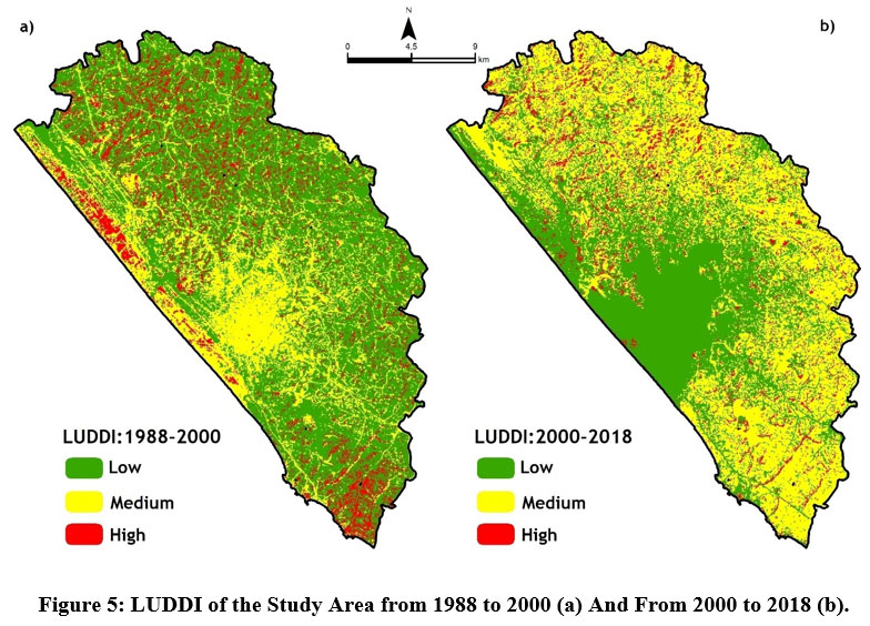 | Figure 5: LUDDI of the Study Area from 1988 to 2000 (a) And From 2000 to 2018 (b).
|
It is also noted that, LUDDI of the 1988-2000 period shows built-up area in medium dynamics index category which is changed into low category in 2000-2018 which indicates that during the time, built-up area expansion is rapid and stable whereas other classes such as agricultural area and SMT and barren land remaining in dynamic nature due to the rapid land use conversion.
Conclusion
In this investigation, geospatial technology is utilized for understanding the LU/LC changes and quantifying the land use dynamics in Thiruvananthapuram city over 30 years from 1988 to 2018. The Landsat imageries of 1988, 2000 and 2018 were used to analyze the LU/LC changes through implementing MLC techniques and results are validated with confusion matrix. The overall classification accuracy is above 85% which is satisfactory. The study reveals that significant LU/LC changes have occurred over the past 30 years. The built-up area rose from 102.08km2 in 1988 to 220.33km2 in 2018 (115.84% increase) and the other land use classes such as barren land, agricultural area, water body and SMT exhibits a declining trend. (i.e., 86.94% ,48.98%, 39.33% and 14.69% respectively). The LUDDI shows that agricultural land together with barren land are the dynamic land uses here. The rapid decline of these land use classes is the outcome of the rapid urbanization and associated land reclamation in the study area. The results are satisfactory and can be of use to local self-governments and planners for making the area green as well as for policy deployments for a scientific and sustainable land use practise.
Acknowledgement
The first author would like to acknowledge the financial support extended by the University Grants Commission by providing the Junior Research Fellowship for doing her PhD (student id:2963/(NET-JUNE2015).
Conflict of Interest
there is no conflict of interest
Funding Source
Funding Source - UGC: JRF (student id:2963/(NET-JUNE2015).
References
- Balsa- Barreiro. J., Li. Y., Morales. A., Pentland A. S. Globalization and the shifting centers of gravity of world’s human dynamics, implications for sustainability. Journal of cleaner production. 2019; 239, p.117923. https://doi.org/10.1016/j.jclepro.2019.117923
CrossRef - Balsa- Barreiro. J., Morales. A. J., Lois- Gonzalez. C. R., Mapping population dynamics at local scales using spatial networks. Complexity. 2021; p. 8632086. https://doi.org/10.1155/2021/8632086
CrossRef - Abebe. G., Getachew. D., Ewunetu. A. Analysing land use/land cover changes and its dynamics using remote sensing and GIS in Gubalafito district, Northeastern Ethiopia. 2021. SN Appl. Sci. 4, 30 (2022). https://doi.org/10.1007/s42452-021-04915-8
CrossRef - Lambin. E.F., Geist. H.J. Dynamics of land-use and landcover change in tropical regions, annual review of environmental resources. 1990. lepers, E., 2003: 28, pp.205-41. https://doi.org/10.1146/annurev.energy.28.050302.105459
CrossRef - Sheeja. R.V., Joseph. S., Jaya. D.S., Baiju. R.S. Land use and land cover changes over a century (1914–2007) in the Neyyar River Basin, Kerala: a remote sensing and GIS approach. International Journal of Digital Earth. 2011; 4(3), pp.258-270. https://doi.org/10.1080/17538947.2010.493959
CrossRef - Patra. S., Sahoo. S., Mishra. P., Mahapatra. S.C. Impacts of urbanization on land use/cover changes and its probable implications on local climate and groundwater level. Journal of urban management. 2018; 7(2), pp.70-84. https://doi.org/10.1016/j.jum.2018.04.006
CrossRef - Anupriya. R.S., Achu. A.L., Rubeena. T.A. Dynamics of Land Use Pattern in the Urban Fringes: A Study of Kazhakkoottam outgrowth of Thiruvananthapuram urban agglomeration. IJRAR. 2019; 6 (2), pp. 504-510.
- Achu. A.L., Reghunath. R., Thomas. J. Mapping of groundwater recharge potential zones and identification of suitable site-specific recharge mechanisms in a tropical river basin. Earth Systems and Environment. 2020; 4(1), pp.131-145. https://doi.org/10.1007/s41748-019-00138-5
CrossRef - Achu., A.L., Thomas. J., Reghunath. R. Multi-criteria decision analysis for delineation of groundwater potential zones in a tropical river basin using remote sensing, GIS and analytical hierarchy process (AHP). Groundwater for Sustainable Development. 2020b.; p.100365.https://doi.org/10.1016/j.gsd.2020.100365
CrossRef - Achu. A.L., Aju. C.D., Reghunath. R. Spatial modelling of shallow landslide susceptibility: a study from the southern Western Ghats region of Kerala, India. Annals of GIS. 2020c; pp.1-19. https://doi.org/10.1080/19475683.2020.1758207
CrossRef - Arulbalaji. P., Padmalal. D., Maya. K. Impact of urbanization and land surface temperature changes in a coastal town in Kerala, India. Environmental Earth Sciences. 2020;79(17), pp.1-18. https://doi.org/10.1007/s12665-020-09120-1
CrossRef - Mansour. S., Al-Belushi. M, Al-Awadhi. T. Monitoring land use and land cover changes in the mountainous cities of Oman using GIS and CA-Markov modelling techniques. Land Use Policy. 2020; 91, p.104414. https://doi.org/10.1016/j.landusepol.2019.104414
CrossRef - UN. (United Nations). World Urbanization Prospects 2018; https://population.un.org/wup/Publications/Files/WUP20 18-Highl ights.pdf
- Nagendra. H., Sudhira. H. S., Katti M., Schewenius. M. Sub-regional assessment of India: Effects of urbanization on land use, biodiversity and ecosystem services. In Th. Elmqvist, M. Fragkias, J. Goodness, B. Güneralp, P. J. Marcotullio, R. I. McDonald, S. Parnell, M. Schewenius, M. Sendstad, K. C. Seto, & C. Wilkinson (Eds.). Urbanization, Biodiversity and Ecosystem Services: Challenges and Opportunities. 2013; (pp. 65–74). The Netherlands: Springer.
CrossRef - Gohain. K.J., Mohammad. P., Goswami. A. Assessing the impact of land use land cover changes on land surface temperature over Pune city, India. Quaternary International. 2020; https://doi.org/10.1016/j.quaint.2020.04.052
CrossRef - Bhagat. R. B. Emerging pattern of urbanisation in India. Economic and Political Weekly. 2011; 46(34), 10–12.
- Heilig, G.K. World urbanization prospects: the 2011 revision. United Nations, Department of Economic and Social Affairs (DESA), Population Division, Population Estimates and Projections Section. 2012; New York.
- Census of India. P. Census of India 2011 Provisional Population Totals. New Delhi: Office of the Registrar General and Census Commissioner. 2011
- John. J., Bindu. G., Srimuruganandam. B., Wadhwa. A., Rajan, P. Land use/land cover and land surface temperature analysis in Wayanad district, India, using satellite imagery. Annals of GIS. 2020; pp.1-18. https://doi.org/10.1080/19475683.2020.1733662
CrossRef - Carlson. T.N., Arthur. S.T. The impact of land use—land cover changes due to urbanization on surface microclimate and hydrology: a satellite perspective. Global and planetary change. 2000; 25(1-2), pp.49-65.
CrossRef - Dewan. A.M., Yamaguchi. Y. Land use and land cover change in Greater Dhaka, Bangladesh: Using remote sensing to promote sustainable urbanization. Applied geography. 2009; 29(3), pp.390-401.
CrossRef - Liu. H., Weng. Q. Landscape metrics for analysing urbanization-induced land use and land cover changes. Geocarto International. 2013; 28(7), pp.582-593.
CrossRef - Yin. J., Yin. Z., Zhong. H., Xu. S., Hu. X., Wang. J., Wu. J. Monitoring urban expansion and land use/land cover changes of Shanghai metropolitan area during the transitional economy (1979–2009) in China. Environmental monitoring and assessment. 2011; 177(1-4), pp.609-621.
CrossRef - Tadese. M., Kumar. L., Koech. R., Kogo. B.K. Mapping of land-use/land-cover changes and its dynamics in Awash River Basin using remote sensing and GIS. Remote Sensing Applications: Society and Environment. 2020; 19, p.100352. https://doi.org/10.1016/j.rsase.2020.100352
CrossRef - Weslati. O., Bouaziz. S., Serbaji. M.M. Mapping and monitoring land use and land cover changes in Mellegue watershed using remote sensing and GIS. Arabian Journal of Geosciences. 2020; 13(14), pp.1-19.
CrossRef - Hakim. A.M.Y., Baja. S., Rampisela. D.A., Arif, S. Modelling land use/land cover changes prediction using multi-layer perceptron neural network (MLPNN): a case study in Makassar City, Indonesia. International Journal of Environmental Studies. 2020; pp.1-18.
CrossRef - S.U Unnikrishnan. A., V. Ashok. S., Reghunath. R., P. T Neena. Land use change detection in Akkulam- Veli lake, Thiruvananthapuram, over the last three decades- An analysis using Remote sensing and GIS tools. IJRASET. 2018: 6 (9), pp. 542-548.
- Government of Kerala. Economic review volume one: State Planning board, Government of Kerala. 2016.
- Iqbal. M.Z., Iqbal, M.J. Land use detection using remote sensing and gis (A case study of Rawalpindi Division). American Journal of Remote Sensing. 2018; 6(1), pp.39-51.
CrossRef - Vivekananda. G.N., Swathi. R., Sujith. A.V.L.N. Multi-temporal image analysis for LULC classification and change detection. European Journal of Remote Sensing. 2020; pp.1-11. https://doi.org/10.1080/22797254.2020.1771215
CrossRef - Lillesand. T., Kiefer. R.W., Chipman. J. Remote sensing and image interpretation. John Wiley & Sons. 2015;
- Kantakumar. L.N., Kumar. S., Schneider. K. Spatiotemporal urban expansion in Pune metropolis, India using remote sensing. Habitat international. 2016; 51, pp.11-22. https://doi.org/10.1016/j.habitatint.2015.10.007
CrossRef - Han. H., Yang. C., Song, J. Scenario simulation and the prediction of land use and land cover change in Beijing, China. Sustainability. 2015; 7(4), pp.4260-4279.
CrossRef - Hassan. Z., Shabbir. R., Ahmad. S.S., Malik. A.H., Aziz. N., Butt. A., Erum. S. Dynamics of land use and land cover change (LULCC) using geospatial techniques: a case study of Islamabad Pakistan. SpringerPlus. 2016; 5(1), p.812.https://doi.org/10.1186/s40064-016-2414-z
CrossRef


