Groundwater Flow Modeling of a Microwatershed using Visual Modflow Flex
Anusha Honnannanavar
 , Nagraj Patil
*
and Vivek Patil
, Nagraj Patil
*
and Vivek Patil
1
Department of Civil Engineering,
Visvesvaraya Technological University,
Belagavi,
Karnataka
India
http://dx.doi.org/10.12944/CWE.18.2.24
Copy the following to cite this article:
Honnannanavar A, Patil N, Patil V. Groundwater Flow Modeling of a Microwatershed using Visual MODFLOW Flex. Curr World Environ 2023;18(2). DOI:http://dx.doi.org/10.12944/CWE.18.2.24
Copy the following to cite this URL:
Honnannanavar A, Patil N, Patil V. Groundwater Flow Modeling of a Microwatershed using Visual MODFLOW Flex. Curr World Environ 2023;18(2).
Download article (pdf)
Citation Manager
Publish History

Introduction
Groundwater is a crucial source that replenishes spontaneously as a result of rainfall and other hydrological processes.1 Nearly all of the earth's subsurface is covered with groundwater. Groundwater is essential for maintaining a healthy ecology, the economy, and human existence.2 Due to its availability and good quality of water; it has become important in all climatic areas. However, with a growing population, increasing industries, and advanced technology in agriculture, most of the recent circumstances of hard rock aquifers in India may have been stressed. All of these actions need daily maintenance in order to return the groundwater resource's state to safe levels.3 Because humans cannot see inside the earth, it is vital to monitor groundwater levels and aquifer parameters on a regular basis in order to comprehend the groundwater flow system. Groundwater models that give insight into the groundwater system have been created for this purpose.3,4 Since it is a crucial source of water to comprehend groundwater flow, conditioning these places as a source of water in semi-arid and drought-prone areas.5 To develop these insights and help make wise judgments, groundwater models may be used. Models are often conceptual representations or approximations that use mathematical equations to explain physical systems and comprehend the environment based on considerations and input values.6 These models could have one, two, or three dimensions, be steady-state, transient, confined, unconfined, or mixed, and be solved using finite difference techniques, finite element methods, or a combination of both.7
In Chikkodi, agriculture dominates the economy. The River Vedganga, which runs through the study region, is a peninsular in India, which falls under a semi-arid region. The major rainfall accounts for the southwest monsoon and in every summer season most of the surface water dried up, which causes water scarcity issues for home and agricultural use for several years.8 In most of these areas, the use of groundwater depends on the crops cultivated on the field and the climatic system using tube wells and dug wells where groundwater extraction is completely necessary. Sustainable management of groundwater resources is crucial and necessitates careful planning to support the growth of agriculture.4 Because of the high demand and heavy withdrawal from the groundwater, it may cause serious damage to the current future water conditions.9 In the presence of groundwater table conditions and a semi-confined environment, groundwater exists within the weathered and fractured Basalt.10 The fact that there is limited information available on groundwater poses a variety of challenges for groundwater assessment in modeling a hard rock region. The current work seeks to comprehend groundwater flow in a typical hard rock region that is bordered by a river despite the recognized limits of the models and high heterogeneity.4
Specifically, because of groundwater development, management, and control of the groundwater problems, it is necessary to improve groundwater in stressed areas.11,12 For these systems, MODFLOW is the best solution as reported by a numerical model developed under steady-state conditions.9 Researchers modeled water budget analysis in Konda -Kalava watershed and Suddegedda river basin. Studies of groundwater at the watershed level are vital for calculating the groundwater budget within the watershed since groundwater development is not constant.13 Hence the present efforts focus on to examine the input and outflow stresses at the micro level under steady-state conditions and also address the groundwater possibilities at the village level using Visual MODFLOW Flex 7.0. For this purpose, a micro-watershed is chosen in Belagavi district.
Study area
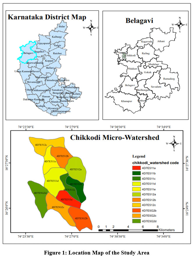
In the Belagavi District of Karnataka's Chikkodi Micro-Watershed, the research was carried out. The area lies roughly between latitudes 16° 23' N and 16° 29' N and longitudes 74° 20' 30" E and 74° 32' 30" E. The micro-watershed covers a total area of 67.52 square kilometers and is situated 18 kilometers west of the Chikkodi taluk. The micro watershed is part of the middle Krishna sub-basin, and its drainage pattern is dendritic to subdendritic.10 From the table.1 there is 696.73 millimeters of rain on average per year. The micro-watershed has a semi-arid climate and geology is made up of banded gneissic complex and basalt. The proposed unruffled weathered rocks, and fractured hard rock under semi-confined conditions. The region is located in Karnataka's Northern Transitional Agro-climatic Zone. The average annual high temperature is 35°C, while the average annual low temperature is 20°C. The minimum and maximum elevations of the zone are 535m and 680m respectively. Vedganga River flows in the study area northeastwards and thereafter joins the Dudhganga River North eastwards and joins the Krishna River at Kallol on the right bank. Agriculture is the primary source of income for 98 percent of the residents in Chikkodi. Maize, jowar, sunflower, wheat, vegetables, cotton, tur, groundnuts, and other major crops are grown when it rains, while paddy and sugarcane, which require a lot of water to grow, are also grown here.
 | Figure 1: Location Map of the Study Area.
|
Groundwater flow model
The most crucial natural resource needed for drinking, irrigation, and industrialization is groundwater. Only when the amount and quality of groundwater are evaluated can the resource be used and sustained in the best possible way.14 The aquifer conditions are predicted and simulated using Modflow. In groundwater modeling, Darcy's law and the continuity equation are frequently coupled. Several models have been developed for groundwater. For the current investigation, Waterloo Hydrogeology's Visual Modflow Flex 7.0 was used to model groundwater flow.
Governing equation of the model,
Where,
.jpg)
Kxx, Kyy, Kzz= The primary axes' hydraulic conductivity (LT-1)
H = Potentiometric head (L)
W = Volumetric flux reflects sources and/or drains of water and is expressed per volume. (T-1)
Ss= Specific storage of porous material (L-1)
t = time (T)
Data used
Meteorological data
The necessary meteorological information for groundwater modeling includes rainfall and recharge. Data about rainfall is gathered from the Statistical Department of Belagavi. A similar technique is used for the research region, according to the National Institute of Hydrology, for the modeling of the Ghataprabha sub-basin, where the recharge value is taken as 15% of the annual rainfall total. The average annual rainfall and groundwater recharge considered for the study is shown in Table 1 and Fig. 2.
Table 1: Rainfall and recharge value from 2015-2019 (Source: Statistical department, Belagavi)
Year | 2015 | 2016 | 2017 | 2018 | 2019 |
Rainfall (mm) | 475.9 | 619.1 | 711.76 | 687.2 | 989.7 |
Initial Recharge (mm) | 71.385 | 92.865 | 106.784 | 103.08 | 148.455 |
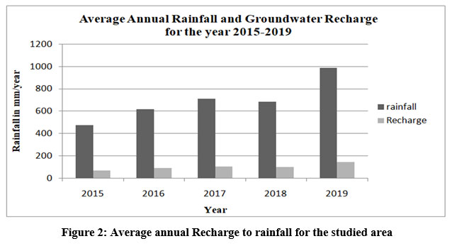 | Figure 2: Average annual Recharge to rainfall for the studied area.
|
Observation well
For ten years from 2010 to 2020, groundwater level monitoring data were collected from CGWB, Belagavi. The locations of the monitoring bore well are shown below in Fig. 3. The elevation of the well in the research area is established with the support of ArcGIS 10.4.1. Data on groundwater levels are processed for modeling purposes. This helps to do trend analysis if there is a decline of groundwater in the selected borewell and an increase in the water level from rainfall recharge and also helps to construct the elevation of different layers more accurately.
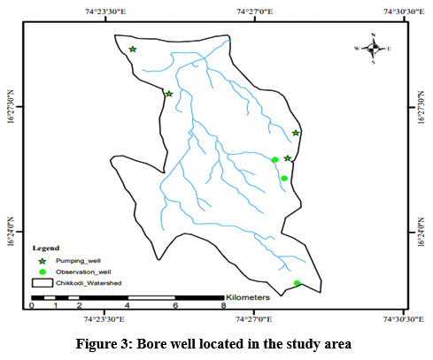 | Figure 3: Bore well located in the study area
|
Methodology
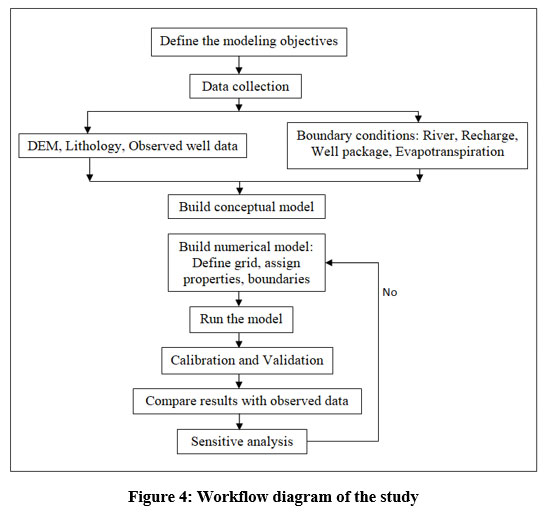
 | Figure 4: Workflow diagram of the study.
|
The conceptual model
The conceptual model, which defines the true extent of the issue and the model's objective, is the initial stage of model development. The development of a conceptual model comes next after the gathering of pertinent data coordinates of bore well locations are taken based on groundwater data from CGWB and imported into the three-dimensional visualization and contouring program SURFER. The model domain has a maximum elevation of 678 m and the lowest elevation of 459 m. This procedure may be carried out using the weighted average distance approach, which makes it easier to comprehend an examination of the area's slope.
Using lithology data and based on the literature review, two geological strata are analyzed and added to the model. The geological top and bottom layers are treated using SURFER software. The first layer of weathered basalt is 30 meters beneath the surface, while the second layer of fractured basalt is 80 meters below the surface as shown in Fig.5.
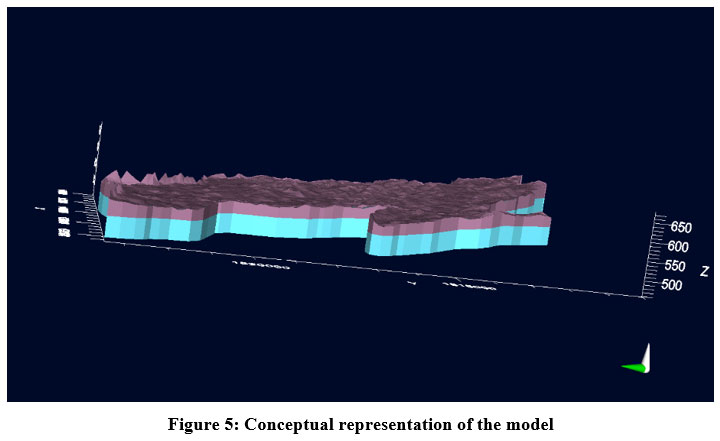 | Figure 5: Conceptual representation of the model.
|
Property zone
For the purpose of building the appropriate zone layers, top and bottom levels are now added to the model. The initial head values, storage properties, and hydraulic conductivity (kx, ky, and kz) are added to each layer's specific layers.
Table 2: Aquifer properties used for model simulation.
Model properties | Values used | |
Hydraulic conductivity (m/day) | Layer 1: Weathered Basalt | Layer 2: Fractured Basalt |
Kx | 1.296 | 0.0399 |
Ky | 1.296 | 0.0399 |
Kz | 0.1296 | 0.00399 |
Storage | Layer 1: Weathered Basalt | Layer 2: Fractured Basalt |
Specific storage | 1.05E-5 | 1.63E-6 |
Specific yield | 0.08 | 0.06 |
Effective porosity | 0.24 | 0.24 |
Total porosity | 0.30 | 0.30 |
Boundary condition
Some of the boundary conditions of the model that are most likely to exist include recharge, streams, reservoirs, evapotranspiration, pumping wells, etc. Due to a dearth of data, these systems were used as boundary conditions in this research.
River boundary condition
For any model to accurately represent how the system interacts with its surroundings, an appropriate set of boundary conditions is required.13 An Arc-GIS interface was used to construct the river's polyline shape file, which was then imported into the model domain.
River thickness (m) | River width (m) | River conductivity (m/day) |
5 | 45 | 0.77 |
Recharge
The recharge package in the visual MODFLOW flex 7.0 includes the recharge values in the model domain. Only precipitation serves as the primary source of recharge in the study area; there are no surface water storage facilities built there. The return flow from irrigation helps the aquifers be recharged. The recharge value is taken constantly for the whole study area. The 15% of the average annual rainfall recharge is taken from the data collected from the statistical department.
The GEC15, states that the formula may be used to calculate recharge,
Recharge=Specific Yield × Geological Area ×Water Table Fluctuation
Evapotranspiration
The actual evapotranspiration is equal to or less than the potential evapotranspiration.9,13 Due to the complexity of the AET computation, PET is taken into consideration. The Hargreaves technique is used to compute PET. In contrast, temperature datasets are extracted using an IMD converter after being obtained from the Indian Meteorological Department (IMD) of the relevant study area. Minimum and maximum temperatures are necessary for the estimate of evapotranspiration when using the Hargreaves technique. The evapotranspiration calculated from the year 2010-2020, the real on average annual ET is 3.4071 mm/day.
Pumping well condition
Pumping well data are collected from Central Ground Water Board, Belagavi. At the community level, the bore wells' pumping or outflow rates are considered. The period of April 2020 is taken for the simulation of the model. The model imports estimated pumping rates expressed in lpm (liters per minute). Microsoft Excel sheet is imported into the model domain. The good data adjacent to the study area are taken into consideration.
Define model grid
By specifying the grid or mesh, a model transforms the conceptual model into a numerical model. Based on the literature research, the study's study area consists of 20 rows and 20 columns, with cells that are 440.247 m in width and 674.412 m in height.
Translation of the model
By choosing the appropriate grid type, the model must be transformed from conceptual to numerical, after which it must be translated and replicated using all of the given inputs, including boundary conditions and reported wells.
Results and discussion
Steady-state calibration
In this model's development, steady state calibration involved comparing hydraulic head simulations from MODFLOW to the measured aquifer heads. 17 observation wells that were observed during April 2020 were used for the calibration. The groundwater model in the Ghataprabha Hiranyakeshi watershed was simulated using a transient case study.3 Here the model has been calibrated to account for recharge, evapotranspiration, and hydraulic conductivity. Because this well governed by significantly greater inferences, it has a high residual error of -10.5 m at the observation well in Chikkodi Village and the 0.053 m lowest residual error is attained (Fig. 6). In the steady state calibration, the lowest RMS error of 5.34 m and NRMS error of 13.23% are attained. As a result, the plot of the observed and estimated head is quite near.
April 2020 marked the completion of the steady-state calibration. The predicted groundwater heads for the micro-watershed reflect patterns of reported groundwater heads in calibration output. According to the zone budget analysis, the basin's total inflow and outflow are 28289.192 and 28290.05 m3/day, respectively. As a result, the basin has a 0.8358 m3/day deficit.16 Artificial recharge structures must be established at potential locations in and around communities in the Chikkodi watershed, taking into consideration the water table decline and groundwater flow patterns of the watershed, in order to increase the groundwater level in the southern part of the watershed.13 The subsequent parts describe the in-depth zone budget analysis and sensitivity analysis.
Water budget
In order to compute water budgets for desired areas in the model, the U.S. Geological Survey built a zone budget tool. To determine the water balance and inflows of the given components into the aquifer system, this research used the zone Budget tool.9 The mass balance technique is used to account for the sources and sinks of the water flowing into and out of the basin region.
Using the zone budget, Table.3 displays the groundwater budget for the entire watershed calculated from the groundwater flow model. In this case, the watershed receives 20518.526 m3/day of daily recharge from rainfall and input to the river leakage of 7770.666 m3/day. Regarding evapotranspiration, a total of 11602 m3/day departs the watershed; while a total of 3023.56 m3/day escapes from the wells. Thus, 28289.192 m3/day of water total enters the watershed every day, while 28290.05 m3/day of water total left the watershed every day. River leakage inflow is greater than river leakage outflow. River leakage accounts for 28.72% of yearly groundwater recharge. The output shows that there is very little storage. To save the groundwater for later use, it is necessary to make prompt arrangements for its recharging using every available method.
Sensitive analysis
Numerous modeling goals, including the analysis of various groundwater flow patterns, the estimation of leakage losses from surface water bodies, the calculation of water table gradients for local issues, and the simulating of flow directions, are frequently addressed by the steady-state solution alone.17
Trial-and-error changes to the steady state calibration may be performed to minimize the Root Mean Square (RMS) errors at the target. By adjusting the hydraulic conductivity of the area and the derived recharge values, steady state calibration is carried out. That initial stratum's estimated hydraulic conductivity is 1.296 m/day, and its subsequent stratum is assessed to be 0.0399 m/day. During the sensitivity study, hydraulic conductivity and recharge values are more sensitive than evapotranspiration, which are discovered in this situation.
Initial sensitivity analysis is conducted using the hydraulic conductivity values.13 During the first sensitivity test, the conductivity values are raised by 10% of the initial calibrated model by keeping the recharge values.16 With this change, the NRMS error rose from 11.20 to 14.2%. Additionally, the conductivity values are reduced by 10% in the second sensitivity experiment. As a result, the NRMS number increased once again to 14.6%. The conductivity value is unaltered, however, the second parameter, Recharge, has been modified. Recharge is once more reduced by 10% for the whole watershed while maintaining consistency with all values, and the NRMS value is subsequently modified from 11.10%. Dry cells in the southern half of the Chikkodi basin area are caused by further reductions in recharging. Excessive groundwater use will result in decreasing groundwater levels in the area if surface evapotranspiration and river leakages of groundwater are continued.
Table 3. Output of the zone budget analysis
Boundary condition | Inflow (m3/day) | Outflow (m3/day) | Outflow as percentage of recharge (%) |
Recharge | 20518.526 | 0 | 0 |
River leakage | 7770.666 | -13664.49 | 28.72 |
Wells | 0 | -3023.56 | 14.73 |
Evapotranspiration | 0 | -11602 | 56.54 |
Total | 28289.192 | -28290.05 | - |
Inflow-Outflow | -0.8358 | ||
 | Figure 6: Calculated and observed head in steady state calibration
|
Conclusion
Our investigation comprises state calibrating for the Chikkodi micro-watershed. Asa consequence, assuming steady-state conditions, three-dimensional subsurface flowing models are being built via Visual MODFLOW Flex. A two-layered conceptualizing is being performed forth by lithology & extensive bibliographic review. This initial stratum comprises of weathered basalt range 30 meters off its surface, whilst the following stratum contains a fractured basalt section 80 meters beneath the surface.8 Package enabling recharging, evapotranspiration, rivers, plus wells were appended onto the experimental area's perimeter conditions. This model's investigation phase calibrating is achieved by employing (17) observable wells. Since evidence is deficient, wells beyond the assigned research districts are covered as the borderline condition, so whatever this sucking well demands in form of statistics is transferred into the research region. The overall intake of the aquifer system is 28289.192 m3/day, while the total outflow is 28290.05 m3/day.9 These findings reveal a 0.8358 m3/day drop in groundwater flow. Cumulative groundwater appropriation through river seeps accounting up estimated 28.72% of the whole groundwater recharge, however, evapotranspiration losses account for approximately 56.54% of the total groundwater recharge.9
Although the region falls within the safe range of groundwater zones, the observed trend of groundwater depletion needs to be considered as an indication for adopting measures for groundwater recharge. Constructing surface water storage facilities such as check dams, and percolation tanks that contribute to future recharge conditions being better. Enhancing the groundwater model's accuracy and addressing the data constraint, particularly in the input boundary condition, are the main objectives of this study. The model is more reliable results with observed and calculated data. For accurate water resource estimation used in improved and more effective water resource planning and management, research of a similar nature might be conducted in other water-stressed locations.
Acknowledgement
Authors thank the Department of Civil Engineering, Visvesvaraya Technological University, Belagavi for providing the facilities to do this work.
Conflict of interest
Authors declare that there is no conflict of interest.
Funding Sources
There is no funding or financial support for this research work.
References
- Varghese AA, Raikar R V, Purandara BK. SIMULATION OF GROUNDWATER LEVELS IN MALAPRABHA. Int J Adv Sci Eng Technol. 2018;(1):30-35.
- Gleeson T, Wada Y, Bierkens MFP, Van Beek LPH. Water balance of global aquifers revealed by groundwater footprint. Nature. 2012;488(7410):197-200. doi:10.1038/nature11295
CrossRef - Patil NS, Chetan NL. Groundwater modeling of Hiranyakeshi watershed of Ghataprabha sub-basin. J Geol Soc India. 2017;90(3):357-361. doi:10.1007/s12594-017-0724-6
CrossRef - Varalakshmi V, Venkateswara Rao B, SuriNaidu L, Tejaswini M. Groundwater Flow Modeling of a Hard Rock Aquifer: Case Study. J Hydrol Eng. 2014;19(5):877-886. doi:10.1061/(asce)he.1943-5584.0000627
CrossRef - Guihéneuf N, Boisson A, Bour O, et al. Groundwater flows in weathered crystalline rocks: Impact of piezometric variations and depth-dependent fracture connectivity. J Hydrol. 2014;511:320-334. doi:10.1016/j.jhydrol.2014.01.061
CrossRef - Sridhar N, Ezhisaivallabi K, Poongothai S, Palanisamy M. Groundwater Flow Modelling Using Visual MODFLOW-A Case Study of Lower Ponnaiyar Sub-Watershed, tamilnadu, India. Int J Eng Res Mech Civ Eng. 2018;3(2):2456-1290.
- Todd, David; Mays L. Groundwater Hydrology. Published online 2001:280-281. http://water.usgs.gov/pubs/circ/circ1186/html/gw_effect.html
- Patil NS, Dhungana S, Purandara BK. Assessment of groundwater in Ghataprabha sub-basin using visual MODFLOW flex. Int J Earth Sci Eng. 2016;9(4):1376-1382.
- Kumar GNP, Kumar PA. Development of Groundwater Flow Model Using Visual MODFLOW. Int J Adv Res. 2014;2(6):649-656.
- Central Ground Water Board Government of India. AQUIFER MAPPING AND MANAGEMENT OF GROUND WATER RESOURCES CHIKKODI TALUK, BELAGAVI DISTRICT , KARNATAKA. 2017;1(1):14. http://cgwb.gov.in/AQM/NAQUIM_REPORT/karnataka/2022/Belagavi District/Chickodi_Belagavi_report.pdf
- Prabhu N, Inayathulla M. A groundwater modeling on hard rock terrain by using visual modflow software for Bangalore North, Karnataka, India. Int J Innov Technol Explor Eng. 2019;8(12):1473-1478. doi:10.35940/ijitee.L3089.1081219
CrossRef - Singh RD, Tyagi JV, Kumar SVV, Rao YRS. NIH / CS / 12-13 Groundwater Flow Modeling in D1 and D2 Disributaries of Left Main Canal under Talluru Lift Scheme of Pushkar Canal System National Institute of Hydrology Deltaic Regional Centre Kakinada.; 2013. http://117.252.14.250:8080/jspui/handle/123456789/5019
- Satyaji Rao YR, Siva Prasad Y. Groundwater flow modeling - A tool for water resources management in the khondalite and sandstone formations. Groundw Sustain Dev. 2020;11:100454. doi:10.1016/j.gsd.2020.100454
CrossRef - Khadri SFR, Pande C. Ground water flow modeling for calibrating steady state using MODFLOW software: a case study of Mahesh River basin, India. Model Earth Syst Environ. 2016;2(1):1-17. doi:10.1007/s40808-015-0049-7
CrossRef - Central Ground Water Board (CGWB), Delhi NEW, Guidelines D, et al. Dynamic Ground Water Resources of India (As on 31 March 2011). Ground Water. 2017;(March 2011):308. https://www.wbidc.com/images/pdf/circular/Water_Industries.pdf%0Ahttp://cgwb.gov.in/Documents/Dynamic GWRE-2013.pdf
- Prasad YS, Rao YRS. Groundwater flow modelling of a micro-watershed in the upland area of East Godavari district, Andhra Pradesh, India. Model Earth Syst Environ. 2018;4(3):1007-1019. doi:10.1007/s40808-018-0502-5
CrossRef - Kareem HH. Study of Water resources by Using 3D Groundwater Modeling in Al-Najaf Region Iraq. Published online 2018:14-15. https://orca.cf.ac.uk/111826/1/Hayder Hatif Kareem Thesis.pdf


