Current World Environment

Introduction

Hydroinformatics focus on applications of advanced information technologies and statistical tools for better understanding and management of the hydrological phenomenon. Hydrological phenomenons are cyclic and stochastic in nature. In hydroinformatics the river is considered as a water-based asset, with flows patterns largely as stochastic. River can be considered both as a generic object with properties pertaining to the flow behavior and as a particular object with its own unique characteristics. The significant information needed for river flood management is about past and present runoff in the river and the governing rainfall data covering the river catchment area coupled with the derived information about the human dimension, the historical, sociological, legal, economic and even political aspects (Patel and Shete, 2007).

The physical models are most efficient to estimate a flood event because such models have built within it knowledge of the physics, like the dimensions of the flood plains, variations in meteorological parameter, runoff coefficients, roughness values, head losses, etc.. However, when there is a need for very rapid predictions of flow patterns, say, in a forecasting situation, or when long time series are being run, or a Monte Carlo analysis is required, then the physicallybased model is cumbersome (Beven, 2001). There are now a number of such situations where time series analyses are being used to forecast such extreme events in rivers. Time series analysis allows identification of hidden deterministic behavior and thus understanding of cause and effect relationship in problems (Schwartz and marcus1990). The univariate model provides an increased understanding of the behavior of the system. The changes in the measured values are the function of shocks (the deviation from the expected results provided system dynamicsheld constant) to the time process occurring during the past months. So that the residuals are not correlated more than 5% insignificant level and normalize the residuals as much as possible. Thus the fitted model is the better choice (Murray and Farber, 1982).

The paper attempts to describe the occurrences of the river floods using stochastic time series forecasting method. The particular emphasis has been given for the accurate flood forecasting and warning for an effective management of flood disaster if required. The form of modeling used to make sense of the acquired data is Time Series ARIMA modeling. The results of an analysis of acquired and generated information supports decision to regulate the real world, the river, its environments and the people associated with it.

Study Area and Data

The applicability of data based stochastic analysis is studied for a perennial medium size hilly river named Kulfo. The river spans in great Abaya - Chamo basin of southern Ethiopia. The Abaya - Chamo basin has a catchments of about 16,400 square kilometers with river drain area consisting of about 3500 square kilometers. Rainfall pattern is mostly indefinite imparting frequent inundation to Kulfo river basin despite an average yearly rainfall figure. The river has response time of about six to eight hours depending upon the rainfall intensity.

For development of the flood forecast model at least one set of continuous flow measurement in each sub-catchments associated with a significant risk area, capable of capturing extreme flood discharges is desirable. Further, a standardized recording of key information, facilitating quick flood response should be maintained. In order to simplify the study only two hydrological variables are selected for the analysis. Data pertaining to the rainfall has been collected from Meteorological Station situated within 1 km range of river and river flow has been measured at rain gauge installed at river discharge point near Abaya Lake. The time plot of individual rainfall Mean Monthly Rainfall (MMR) and Mean Monthly Discharge (MMD) time series have been given in fig 1 in a comparable form to reveal quantitative consistency of MMD with MMR data set. The data ranges have been taken as monthly cumulative and eight year data beginning from January 1990 and continuing till the end of 1998.

Fig. 1 shows an examination of the quality of data base and the degree of independence for each variable. From these plots we infer that the data behave in a normalized manner and spread in data is uniform over the time with cyclic nature. The relationship between rainfall and river discharge is linear or very nearly so. There is some inconsistency in observed data towards the end of year 1996, where the runoff and rainfall are not concurrent in terms of quantity. The exact reason for which cannot be inferred however, the gap may be attributed to observational mistake or sudden release of dammed water.
 

Figure 1: Rainfall and runoff of Kulfo River (Jan. 1990 - Dec. 1998) Click here to view figure

Methodology of Model Development

Real time flood forecasting can be done using statistical, stochastic, deterministic and soft computing techniques. When the occurrence and outcome of a phenomenon, as in natural processes, are random or uncertain the process is characterized as stochastic (Priyan and Dalwadi, 2007). In hydrological phenomenon the rainfall is the main occurrence with runoff as its foremost associated outcome. Both rainfall and runoff are function of space and time and are covary geographically and temporarily (and seasonally). Therefore, the flood which too is a consequence of rainfall and runoff can smartly be represented and forecasted by use of stochastical modeling of historical runoff data. Stochastic model are good enough to capture sudden changes in natural flood however the gaps in flood data impair forecasting results.

The observation of rainfall and runoff taken at temporal order constitute the time series. The inherent cause effect relationship in the hydrological phenomenon of a stochastic time series can be analysed by applying of the Box – Jenkins approach (Box and Jenkin, 1994). The Box- Jenkins approach usages the concept of AutoRegression Integration and Moving Average (abbreviated as ARIMA) modeling, where the dependent variable is lag regressed onto itself and smoothened thus giving rise to the ARMA and related ARIMA and SARIMA models (S stands for the seasonally regressed time series). These models are applicable to stationary series, where there is no systematic change in mean (i.e. the series has been detrained) and variance is constant over time (Kendall and Ord, 1992).
 

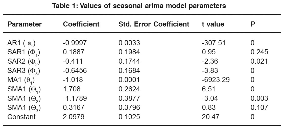Table 1: Values of seasonal arima model parameters Click here to view table

The degree of dependence of variables is analyzed by estimating the autocorrelation function. for MMD series. These results are significant at the 95% confidence level or twice the standard deviation which is 0.068 (using 1/n^½, where n = 84) the total numbers of observed variables. In general a non seasonal ARIMA model can be written as
 

(1₁ B ₂ B ² .. _p B ^p )  ^d z _t =(1- ₁B- ₂ B²-..- _q B^q )a_t

where at, denotes the residual series, B backward shift operator defined as BZ_t = Z_t-1, B²Zt = Z_t-2 and so on and the terms of φ and θ denotes coefficient value of an autoregressive and moving average process of order p and q respectively. When an observation zt of a particular month has some relation with the observation made in the same month of the previous year, the seasonal dependency modify the equation as:

(1 ₁ B ₂ B ^{2 s} .. _p B ^ps )  _s^D z _t =(1-  ₁ B^s -  ₂ B^2s -..-  _q B^Qs )e_t

where et is a normal random deviate, and seasonality s = 12 and the terms given by Θ and Φ, represents corresponding seasonal moving average and autoregressive operators of order Q and P. As et of seasonal ARIMA equation is not necessarily independent, therefore combining non seasonal and seasonal equations we get the general multiplicative seasonal ARIMA model of order (p,d,q) x (P,D,Q) of the form

_p ( B ^s ) _p ( B) _s^D z _t = _Q (B^s )- _q (B)a_t

Results and Discussion

Model Development Process

The objectives of this study are firstly to identify a suitable ARIMA model based on Box-Jenkins approach. Since rainfall and hence river runoff is a seasonal phenomenon, we need to identify the order (p,d,q) x (P,D,Q) for a seasonal univariate model and also to find out the degree of best fit seasonality, which provides a parsimonious representation for both the stochastic component and the total series under consideration. Finally the least square estimates of the parameters of time series models are used for forecasting the river flow. For identification of ARIMA model parameters (p, d, q) and (P, D, Q), the Auto correlations coefficient (ACC) and Partial autocorrelations coefficient (PAC) of MMD time series have been plotted for various combinations of differencing (d=0 and d=1) and lags. The graphical representation of ARIMA model building process is given in the fig. 2. The original and differenced data has been plotted to check the stationarity in the MMD time series. Identification of model parameter is mainly based on ACC and PAC plots of time series. The runoff of the Kulfo River shows a strong seasonal pattern, the same can be seen in the ACC and PACC plots and hence the flow pattern requires a seasonal model.
 

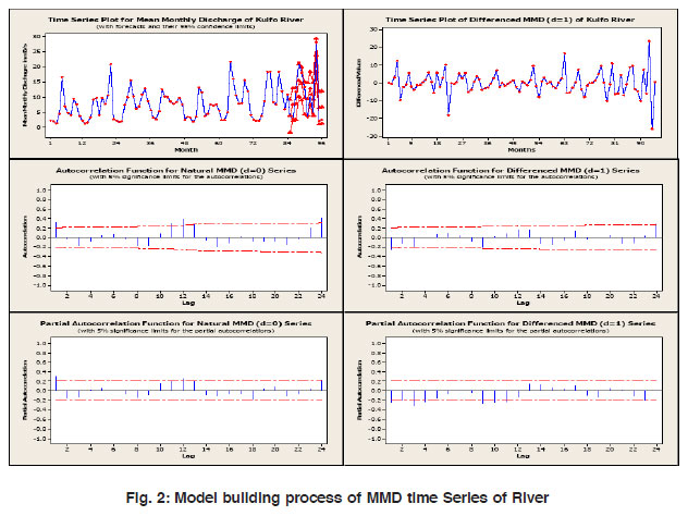Figure 2: Model building process of MMD time Series of River Click here to view figure

An analysis of significant ACC and PAC plots implies to the first order non seasonal ARMA and third order seasonal ARIMA parameterization of MMD series. Compared with 95% confidence limits, few of the partial autocorrelations (three) are found significant. The finally selected seasonal ARIMA forecast model for the mean monthly discharge of Kulfo river is (p,d,q, P,D,Q)S = (1,0,1,3,1,3)12. The other ARIMA model tried with different parametric value could not result in an impressive forecast. In table 1, the values of various AR and MA parameters for seasonal and non seasonal cases are given with corresponding standard error (SE) of coefficient, and t and p values. Small SE coefficient and p value with corresponding t statistic indicate the significance and the preciseness of the coefficient estimation.

 

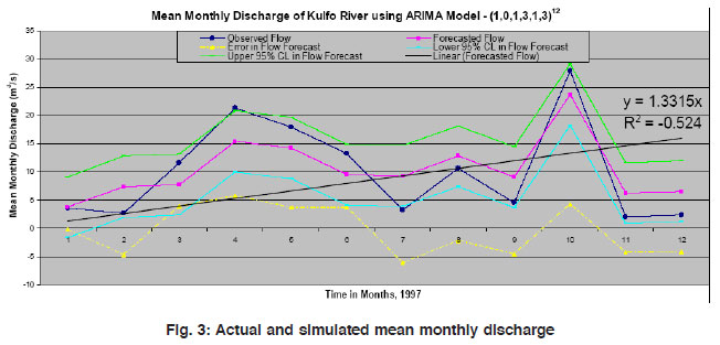Figure 3: Actual and simulated mean monthly discharge Click here to view figure

The fitting of the properly transformed data to the time series model is accomplished by obtaining least square estimate of the parameters. The residuals from the univariate process are used in the final selection of the complete dynamic model. For each iteration / phase of model fitting, the criteria for adequacy of model is that the residuals should be independent (i.e. no or negligible autocorrelation exist) and that the model exhibits parsimony (least number of parameters). The residuals should also exhibit a symmetric distribution (e.g. a normal distribution) (Murray et. al., 1982). The negative values of fitted auto regression parameter explains that the time series variables are related in a quash manner, means their effect is to reduce the discharge value.
 

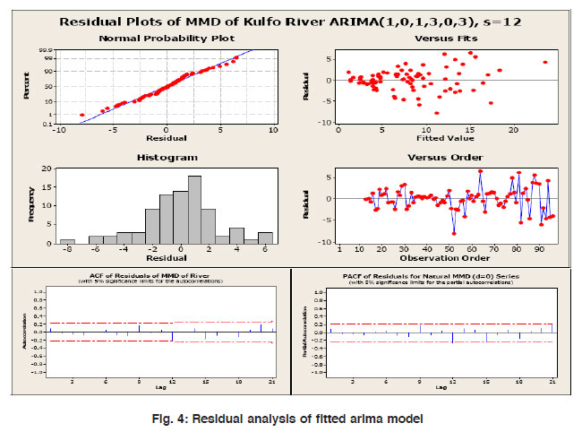Figure 4: Residual analysis of fitted arima model Click here to view figure

The Forecast

The process of creating reliable and robust analysis mostly results in the models of underpredicted extreme river discharge. This is in view of the fact that the computational modeling is limited to situations where the theoretical analysis is valid and sufficient data are available for proper calibration and verification. Monthly runoff discharge is forecasted for 12 months lead time taking January 1997 as the origin. It is obvious from fig. 3 that the results of forecast for all twelve months are reasonably close to the actual river flow and following the mean values. The forecasts are sensibly fair in capturing runoff pattern even in the case of astonishing peaks as in the case of October, 1997. The forecast error equally fall both sides of zero mean value and the forecasted values have a linear increasing trend.
 

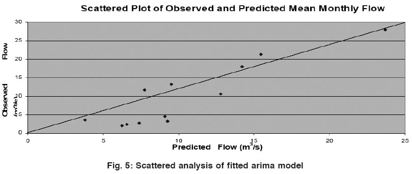Figure 5: Scattered analysis of fitted arima model Click here to view figure

Forecast Evaluation

There are two methods to evaluate the performance of model results first one is using established statistical formulae and the other is stochastic, through the application of data itself i.e. residual analysis. The importance of the later one is justified because it emphasis more to judge the inherent data characteristics. The main advantage of stochastic method is that one can evaluate model performance by the same methods used for model building and any discrepancies in model formulation can be easily recognized so that modeler can take immediate decision for improvement of model. Former one is applicable for all models related to the natural process and are adequately explained in the literature.
 

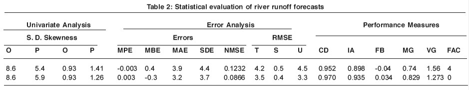Table 2: Statistical evaluation of river runoff forecasts Click here to view table

Preliminary Statistical Evaluation
 

1. ASTM, “Standard Guide for Statistical Evaluation of Atmospheric Dispersion Model Performance,” D6589, American Society for Testing & Materials, Conshohocken, PA 19428-2959 (2000)
2. Beven, J.K., “Rainfall-Runoff Modelling-The Primer,” John Wiley & Sons Ltd., Chichester, 319 (2001).
3. Box, G.E.P., Jenkins, G.M., and Reinsel, G.C., “Time Series Analysis, Forecasting and Control,” third edition, Prentice Hall, Englewood Cliffs (1994).
4. Boyle, D.P., Gupta, H.V., and Sorooshian, S., “Toward Improved Calibration of Hydrologic Models: Combining the Strengths of Manual and Automatic Methods,” Water Resources, AGU, 2000 36(12): 3663-3674.
5. Hanna, S.R. and Chang, J. C., “Air Quality Model Performance Evaluation. Journal of Meteorology and Atmospheric Physics,” (2004) 87: 167-196.
6. Kendall, M., and Ord, J.K., “Time Series, International Journal of forecasting,” (1992) 4: 532-533
7. Legates, D. R. and McCabe Jr., G. J., “Evaluating the use of Goodness-of-Fit Measures in Hydrologic and Hydro Climatic Model Validation,” Water Resource, (1999) 35(1): 233-241.
8. Murray, L.C., and Farber, R.J., “Time Series Analysis of an historical visibility data base,” Atmospheric Environment, (1982) 16(10): 2299-2308.
9. Nigam, S., Kulshrestha, M., Mittal, S., and Singh, K., “Computational Modeling of Air Pollutants in Congested Traffic Condition,” International Conference on Best Practices to Relieve Congestion on Mixed-Traffic Urban Streets in Developing Countries, IIT Chennai, Allied Publisher Pvt. Ltd., India, (2008) 389-400.
10. Patel, N.R., and Shete, D.T., “Probability Distribution Analysis of Consecutive Days Rainfall Data for Sabarkantha District of North Gujrat Region, India”, National Conference on Hydraulics and Water resources, SVNIT, Surat Published by the Elite Publishing House Pvt. Ltd., India, (2007) 86-93.
11. Priyan, K., and Dalwadi, H.J., “Statistical Analysis of Hydrological Data: A study of meghal river basin,” National Conference on Hydraulics and Water resources, SVNIT, Surat Published by the Elite Publishing House Pvt. Ltd., India, (2007) 16-23.
12. Schwarz, J., and Marcus, A., “Mortality and Air Pollution in London: A Time Series Analysis,” American Journal of Epidemiology, (1990) 105: 1273-1281.
13. Willmot, C.J., “Statistics for Evaluation and Comparison of Models,” Journal of Geophysics Research, (1985) 90(5): 8995-9005