Current World Environment

Introduction

Energy extraction from wind involves very complex technology and dynamic nature of wind with continuous changing direction and speed has made the procedure more cumbersome¹. The effects of drag and tip-losses should be taken into account for optimum design and peak performance prediction. Instead of conventional trial and error method to reach maximum elemental power coefficient at a radial station, it should be reached directly through analytical approach². A relationship among two speed interference factors, drag-to-lift factor was derived for maximum elemental power coefficient. With the help of this relationship, the computation for design and peak performance begins directly at peak performance point and the trial and error process is obviated³.

In this study a method evolves computation techniques for designing of wind turbine blade for maximum power production⁴. The turbine simulator is prepared, for determine the value of co-efficient of power Cp and power produce (theoretical) and compared with Wind data collected from study site located at 77°35'E Longitude and 23°28' N Latitudes at the height of 530 m above mean sea level near Bhopal.

Objective of the study

1. New method for optimal design and peak performance prediction.
2. Classification of terrain features including porosity, roughness and obstacles at turbine site.
3. Technical detail of wind Turbine and power curve.
4. Analysis of data collected from Wind Turbine site.
5. Determine Annual Energy Production.

Methodology

For design of the rotor and its peak performance prediction, a blade was divided into 100 radial elements. Total number of 100 radial stations was taken in to consideration. The contribution of power from the inner 5 percent and the outer 5 per cent lengths of the blade were not accounted due to tip loss factor. The blade chord, its twist and elemental power coefficient at each station were determined. Fig.1 show blade divided in 100 elements.
 

Figure 1: Blade of 10kW Horizontal Axis Wind Turbine in 100 Parts Click here to View figure

Speed Interference Factors

The axial and angular speed interference factors, a and a' for a radial station were determined by solving the Eqns

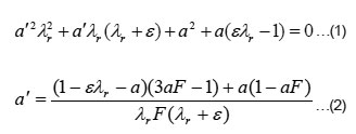
The solution was obtained following Newton-Raphson method [5]. The initial value of 'a' was taken to be 0.30.Through Newton-Rap son method, the functions G1 and G2 were taken as follows:


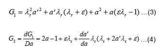
Where da'/da Eqn-      (5)

Eqn- G1 and G2 were determined from Eqns (3), (4) and (5).

i. New value of 'a' was determined as -



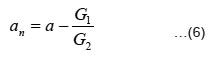
ii. Difference of old and new values of 'a' was computed as -

Da = |a - a_n|

iii. Old value of 'a' was replaced with new value an .

iv. If da ³ 10-5, steps (iii) through (vii) were repeated.

v. For da < 10-5, the values of a and a' were taken as the speed interference factors.
 

Figure 2: Location of Turbine Site at RGPV Bhopal Site and Terrain Features. Click here to View figure.

Chord Length and Twist of Blade

At the given radial station, the relative wind angle φ was determined with the help of Eqn.



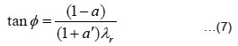
The twist of the blade β is ( φ − α ), where α is the angle of attack for airfoil section of the blade at which the Cd/Cl ratio is minimum⁶.

Solidity Ratio

The local solidity ratio σ from


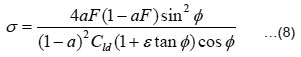
where Cld is the lift coefficient corresponding to minimum Cd /Cl ratio for the given airfoil section. After calculating σ, the chord length was determined with the help of Eqn.



Power Coefficient

The elemental power coefficient at the radial station was determined with the help of Eqn.



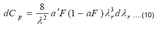
For numerical integration the Eqn. is modified to the following form :


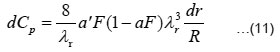
Following Simpson's rule⁸ of numerical integration, the total power coefficient was determined by –



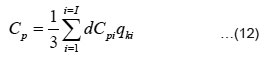
where qki = 3 + (-1)i+1, and I = number of radial stations I = 100
 

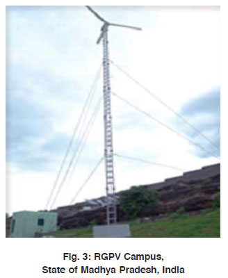Figure 3: RGPV Campus, State of Madhya Pradesh, India. Click here to View figure.

In the new method of optimum design and peak performance prediction, the iterative processes required for convergence of speed interference factors and for maximization of power coefficient through comparison were obviated because of the exact relationship established for a, a', ε and F corresponding to maximum power coefficient⁵. The iterative process required in the new method was only for solution of an equation following Newton-Raphson method which required maximum of 10 iterations for accuracy of 10-5 for 'a'. The design process begins right at maximum power point, rather than searching for point of maximum power and then doing the computations. This has resulted in simplifications of the optimum design and accurate peak power prediction for horizontal axis wind turbine.
 

Table 1: Measures values of properties of obstacles for Turbine at RGPV Hill Click here to View table.

Description of Measuring Site

The topography map No.55 E/7 has been obtained from the Geological Survey of India which shows the contours of hilly site near Bhopal for which the study has been carried out (Fig. 2). The Bhopal under consideration covers an area of approximately 256 square kilometres in undulating topography, interspersed with water bodies, cultivated and barren land and semi urban dwellings. Fig.2 Location of Turbine Site at RGPV Bhopal Site and Terrain Features, and Fig.3 show installed wind turbine at RGPV hill.
 

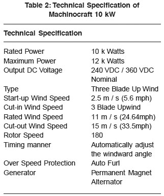Table 2: Technical Specification of Machinocraft 10 kW Click here to View table.

Specifying obstacles near measuring site

Each obstacle present near the measuring site affect the wind data collected and it depend upon porosity and roughness of the terrain. Each obstacle must be specified by its position relative to the site and its dimensions and must be assigned porosity. The position of an obstacle is specified in a local, polar coordinate system. Angles (bearings measured with a compass) are given clockwise from north; distance is the radial length from the site to the corner of the obstacle (measured with a measuring tape or a range finder). Obstacle near turbine site is shown in fig. 3.Table 1 shown the distance of various obstacles.As a general rule, the porosity can be set equal to zero for buildings and ~ 0.5 for trees. A row of similar buildings with a separation between them of one third the length of a building will have aporosity of about 0.33.  
 

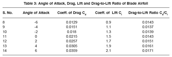Table 3: Angle of Attack, Drag, Lift and Drag-to-Lift Ratio of Blade Airfoil Click here to View table.

Technical detail of Wind Turbine and Power Curve

Machinocraft 10 kW wind turbine generator was installed at hilly site of RGPV located at 77°35'E Longitude and 23°28' N Latitudes at the height of 530 m above mean sea level near Bhopal. Technical specification is shown in Table.2, and power curve shown in Fig.4. The wind turbine rotor made of three propeller type blade. Bushings with internal threads are embedded in the root section, and so forming the attachment to the hub. The shells, spars and root section are made of fiber-glass reinforced polyester, where the main strength properties have been achieved by using continuous fibers (Unidirectional Rowings). The bushings are made of chrome alloy steel. All metal parts for the aerodynamic blade tip brake are made of stainless steel and carbon-fiber and epoxy.
 

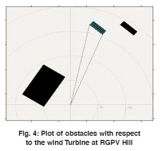Figure 4: Plot of obstacles with respect to the wind Turbine at RGPV Hill Click here to View figure.

Technical Detail of Wind Turbine Blade Measured at site

The profile is NACA 63400 series has proven highly productive and shows little sensitivity to dirt. Also its stalling properties are fine. Each blade in a set normally three blades is balanced to have the same weight in the root as well as tip as the two other blades in the set[9]. The aerodynamic data of blade profile is given in Table 2 and its minimum drag to lift ratio is 0.0137. Angle of attack is -4?. Specification of wind turbine blade is shown in Table 4.
 

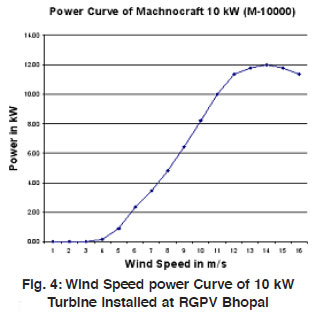Figure 4: Wind Speed power Curve of 10 kW Turbine installed at RGPV Bhopal Click here to View figure.

 

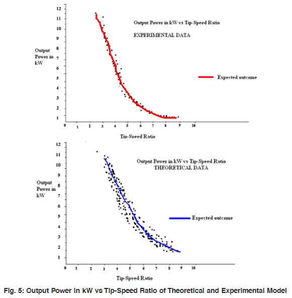Figure 5: Output Power in kW vs Tip-Speed Ratio of Theoretical and Experimental Model Click here to View figure.

Analysis of Experimental data collected from Wind Turbine site

Data are recorded in data loger, set for one month time duration reading at every 1 min interval give us information about wind speed and power generation. Recorded data is further presses to find out tip speed ratio (?) and coefficient of power (Cp) by above formula. Table 5 show the experimental data collected from turbine site.

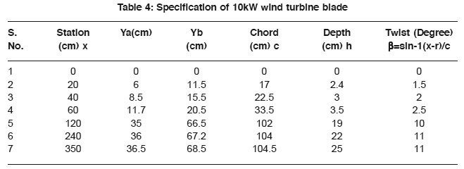Table 4: Specification of 10kW wind turbine blade. Click here to View table.

Results and Discussion

To design a wind turbine rotor blade chord, its twist and its elementary power co-efficient at each station were determined. The iterative process required for the convergence of speed interference factor and for maximization of power coefficient through comparison were obviated because of exact relationship establish for axial interference factor (a), angular speed interference factor (a'), Cd/Cl ratio (ε) corresponding to maximum power coefficient. It is found that on wind rotor runs at optimum design condition. There is variation in wind speed and angle of attack. The consideration of tip-loss correction factor (F). In the above Example the power generated by blade profile and same can be calculated for other NACA profil.
 

Table 5: Experimental Data Collected from Turbine Site. Click here to View table.

 

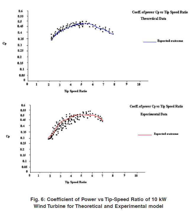Figure 6: Coefficient of Power vs Tip-Speed Ratio of 10 kW Wind Turbine for Theoretical and Experimental model. Click here to View figure.

Results are generated from the data collected from study site as these data are applied on mathematical model based on new method for optimal design and peak performance prediction by this generating the value of coefficient of power Cp and power produced theoretical and Experimental shown in the figure 5 and 6. The maximum power is generated when l is between 2.8 – 4 and the maximum value of Cp (0.45) is obtained when the tip speed ratio (l) is 3-4.The figure 5 and 6 shows the experimental results come out maximum power generated by the turbine is in between 7-10 KW where l is in between 3-4.

Show experimental power generated by WEG. By integrating the theoretical and experimental data results are come out, the theoretical power generated by mathematical turbine simulation comes out 60.25 kWh and experimental power generated 42.85 kWh.
  

References

1. Griffiths, R.T. and M.G. Wollard, Performance of the optimal wind turbine, Journal of Appl. Energy, (1978) 4: 261-272
2. Glauert, H., Airplane propellers in Aerodynamic Theory. Ed. Durand, W. F. Dover Publications, New York (1963).
3. Jones, C.N., Blade element performance in horizontal axis wind turbine rotors, Int. Journal of Wind Engineering, (1983) 7(3): 129-137.
4. Jansen, W.A.M., Horizontal axis fast running wind turbines for developing countries. SWD 76-3, Steering Committee for Wind Energy in Developing Countries, Amersfoort, The Netherlands, (1976) 91.
5. Riegler, G., Principles of energy extraction from a free stream by means of wind turbine, Int. J. of Wind Engg., (1983) 7(2): 115-125.
6. Rohrbach, C., H. Wainauski and R. Worobel, Experimental and analytical research on aerodynamics of wind driven turbines, Hamilton Standards, Division of United Technologies Corpn., Connecticut, (1977) 250.
7. Sastry, S.S., Engineering mathematics, 2, Prentice Hall of India (2003).
8. Stevens, M. T. M. and P. T. Smulders, "The Estimation of the parameters of the Weibull wind speed distribution for wind energy utilization purposes", Int. Journal of Wind Engg., (1999) 3(2): 132-14.