Sodium Adsorption Ratio (SAR) Prediction of the Chalghazi River Using Artificial Neural Network (ANN) Iran
Gholamreza Asadollahfardi1 * , Azadeh Hemati2 , Saber Moradinejad1 and Rashin Asadollahfardi3
1
Semnan Regional Water Company,
Semnan,
Iran
2
Civil company,
Vancouver,
Canada
DOI: http://dx.doi.org/10.12944/CWE.8.2.02
Copy the following to cite this article:
Asadollahfardi G, Hemati A, Moradinejad A, Asadollahfardi R. Sodium Adsorption Ratio (SAR) Prediction of the Chalghazi River Using Artificial Neural Network (ANN) Iran. Curr World Environ 2013;8(2) DOI:http://dx.doi.org/10.12944/CWE.8.2.02
Copy the following to cite this URL:
Asadollahfardi G, Hemati A, Moradinejad A, Asadollahfardi R. Sodium Adsorption Ratio (SAR) Prediction of the Chalghazi River Using Artificial Neural Network (ANN) Iran. Curr World Environ 2013;8(2). Available from: http://www.cwejournal.org/?p=4531
Download article (pdf) Citation Manager Publish History
Select type of program for download
| Endnote EndNote format (Mac & Win) | |
| Reference Manager Ris format (Win only) | |
| Procite Ris format (Win only) | |
| Medlars Format | |
| RefWorks Format RefWorks format (Mac & Win) | |
| BibTex Format BibTex format (Mac & Win) |
Article Publishing History
| Received: | 2013-04-25 |
|---|---|
| Accepted: | 2013-06-12 |
Water quality management is the surface water and groundwater quality control at any time for supplying water at a required quality for a specific use. Long-term strategies for national water resources development in a country is based on water supply, demand management, water reform, compliance with environmental aspects, and finally management of the water consumer’s activities. Identifying and estimating the basic parameters which affect the quality of water resources helps in implementing policies and strategies. River quality control requires additional investment for wastewater treatment and collection systems. On the other hand, it may lead to restricted development in the basin and could have a significant economic impact. For water quality control it is necessary to know physical, chemical and biological characteristics of the river. To reach this objective, it is necessary to have proper monitoring of water quality. Having enough data without proper interpretation cannot help water quality management adequately. There are several methods for analyzing water quality data, such as statistical models, deterministic models and artificial neural models Asadollahfardi et al. (2011 - 2012) . Dogan et al., (2007) used the ANN to forecast BOD concentration using data from eleven stations on the Melen River in 2001-2002, including COD, temperature, DO, chlorophyll-a, ammonia, nitrite and nitrate. They concluded that the ANN model provides a reasonable estimate for BOD parameter. Singh et al., (2009) applied the ANN to predict dissolved oxygen and BOD using ten years of data at eight different stations in India. The input of the model consisted of eleven monthly water quality parameters, and the predictions and actual data had a good agreement. Huang and Foo (2002) applied the ANN for the assessment of the variation of water salinity in the Apalachicola River in Florida. They employed part of existing data for testing and the remainder of the data for the validity of the ANN model. Maier and Dandy (2002) reported 41 successful case studies of prediction of water changing, which uses the MLP neural. Coppola et al., (2003) described the successful application of the technology for three kinds of management and underground water prediction. In the first instance, an ANN was trained by simulation of data collected from a numerical model based on physical data in the appropriate places, with various pumping and climate conditions. The ANN obtained a high precision for forecasting, and its altering statue equations were substituted in the multipurpose optimal formula. In the second and third instances, the ANNs were developed according to climate and hydrology real data for the different environmental hydrology conditions. For the second problem, an ANN was developed using the information collected over five years and eight months and under various climates and pumping conditions to predict the heights in a limestone and ice layer under the multi-layer soil.
Misaghi et al. (2003) studied water quality in the Zayandeh Rud River applying a General Regression Neural Network (GRNN) for ten years of BOD and DO. Musavi-Jahromi and Golabi (2008) applied the ANN to monthly water quality of the Karoon River, Iran, using CO, HCO3-, SO4, CL, Na, Ca, Mg and K as inputs and TDS, EC and SAR as outputs. Their results were satisfactory. Kanani et al. (2008) studied water quality in the Achechay River, but they selected a water quality monitoring station and applied MLP and Input Delay Neural Network (IDNN) models. They predicted TDS parameters using discharge as input data to the models. Olyaie et al. (2010) employed the MLP model with water quality parameters including BOD and DO in Hamadan Morad Beik River. Their outcome was satisfactory. Asadollahfardi et al. (2010) applied the MLP model to total phosphor and total nitrogen data in an Anzaliy Wetland (Iran) study and obtained acceptable prediction for eutrophication in the wetland. Asadollahfardi et al. (2012) applied the MLP and Elman dynamic of the ANN to two stations of Talkheh Rud River and predicted TDS of the river one month in advance, and the results were acceptable. Generally for assessment of the dispersion risk of irrigation water it is significant to consider the ratio of sodium to other exchangeable cations on soil colloids. High sodium ions in water affect the permeability of the soil and cause of infiltration problems. When sodium exists in the soil in an exchangeable form, it replaces the calcium and magnesium absorbed on the soil clays and causes dispersion of soil particles. The SAR has a proper criterion for irrigation water suitability. If calcium and magnesium are the predominant cations absorbed on the soil exchange complex, the soil tends to be easily cultivated and has a permeable and granular structure Asadollahfardi et al. (2010).
Zhang and Stanley (1997) using the artificial neural network (ANN) modeling technique were used to establish a model for forecasting the raw-water coloring in a large river. In this research the potential applications of ANN in the water treatment industry are also discussed. Results indicate that the ANN modeling scheme shows much promise for water quality modeling and process control in water treatment. Keiner and Yan (1998) studied sea Surface Chlorophyll and Sediments from Thematic Mapper Imagery using neural network models. It was found that a neural network with two hidden nodes, using the three visible Landsat Thematic Mapper bands as inputs, was able to model the transfer function to a much higher accurately than multiple regression analysis. The RMS errors for the neural network were <10%, while the errors in regression analysis were >25%. Zhang et al. (2002) studied water quality in the Gulf of Finland using an empirical neural network and combined optical data and microwave data. The results showed that the estimation accuracy of the major characteristics of surface waters using the neural network is much better than those from the regression analysis.
The study area is a part of the Sirwan Basin with a total area about 105,000 hectares which contain 3.8% of the Kurdistan provincial area. The north of the basin is surrounded by the Sefed River catchment area, east of the area is the Ghaveh River, and west of the area has a common boundary with the Seravan River. The catchment is located between 46°, 46', 40" and 47°, 20', 00" East longitude and 35°, 24', 44" and 35°, 43', 23" North latitude (Figure 1).
The height of the area varies from 1500 to 2900 meters. All of the surface runoff of the basin is collected by the Chelghazy and Khalefeh Tar Khan main river (Mohammady and Fathi, 2004). Figure 1 shows the study area. The weather conditions of the basin are similar to subtropical dry region weather. Its winters are cold; its summers are relatively warm and dry, and its rainy season is from October to May. The average annual minimum and maximum temperatures between 1990 and 2005 were 6.3 and 21.8 degrees Centigrade, respectively. The average annual minimum and maximum humidity between 1990 and 2005 was 26.7% and 21.8%, respectively. The annual total rainfall was 395 mm, Islamic Republic of Iran Meteorological Organization (1983). The basin is part of the Kurdistan Province, which is geologically quite active. The land straddles the seduction zone between the colliding Eurasian and African tectonic plates. Locally, the breakaway Arabian micro plate is being sub ducted under the Iranian and Anatolian Micro plates at the rate of a few inches a year, and as a result the Zagros mountains and Kurdistan—the point of this collision—are being compressed and pushed upward several inches a year (Hooshmand Zadeh, 1995).
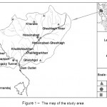 |
Figure 1: The map of the study area. Click here to View figure |
The high concentration of sodium in irrigation water may negatively affect the soil structure and decrease the soil hydraulic conductivity in fine-textured soil. The degree to which sodium will be absorbed by a soil is a function of the amount of sodium to divalent cations(Ca and Mg) and is regularly stated by the sodium adsorption ratio(SAR) (Bouwer and Idelovitch 1987). The SAR is a general water quality index that indicates the percentage of sodium in the water and function of the ratio of sodium to divalent cations such as Ca and Mg. The SAR parameter is obtained from the Eq. (1). (Asadollahfardi et al., 2011):


Where pk2=negative logarithm of the second dissociation constant for carbonic acid; pkc=solubility constant for calcite; and p=negative logarithm of ion concentration (meq/L). The amount of p (k2-KC), p (Ca+Mg) and p (Alk) related to Ca+++Mg+++Na+, Ca+++Mg++ and +HC respectively can be found in Bouwer (1974).
The adjusted SARadj value typically is computed, which take into account the effects of rainfall. Sodium also has adverse effects on the crops such as leaf burn in almond, avocado, and stone fruits (Bouwer and Idelovitch 1987). Ayers and Tangi (1981) suggested that whether the SARadj water for irrigation is below 3, there are no sodium problems if the SAR is between 3 and 9 there are increasing problem and whether the SAR is above 9, there are severe problems. The first objective of this study was set to develop an ANN-based prediction model for monthly SAR. Development of the model uses the discharge, sodium, calcium, magnesium, chloride, sulfate, bicarbonate, pH and SAR data for a station of the Chalgazi River Basin in the Kurdistan Province, which were collected from the Water Authority of Kurdistan. The second aim was using sensitivity analysis to find out which of the mentioned parameters were significant in the prediction of the SAR.
Methodology
The ANN is a data processing system, based on an idea similar to the processing of the human brain that treats data as a steady network parallel to each other in order to solve a problem. With the networks, the structure of data is designed to help programming knowledge in which the behavior is the same as natural neural and its component. An artificial neural system consists of three components, including weighting (W), bias (b) and transfer function (f). These three components are unique to each neural system. In Figure 2, “p” and “n” equal input and output while “a” equal net input. The junctions of 1 and 2 in Figure 2 show the schematic of the artificial neural system. The function of artificial neural network would be called “p”.


The MLP is a static neural network which has three layers including an input layer, hidden layer and output layer.
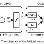 |
Figure 2: The schematic of the Artificial Neural Network (ANN) Click here to View figure |
Figure 2 shows the schematic of the ANN. Figure 3 shows schematically tangent – sigmoid transfer function and linear transfer function. Number of neurons in the hidden layers for each model may be obtained using trial and error. The function of the network can be modeled by equations 5 and 6 (Menhaj, 1998):


Where, R = numbers of input vector components. S1 and S2 = numbers of neurons in hidden and output layers, respectively. P = input vector. W1 and w2 = weighting matrix in hidden and output layers, respectively. b1 and b2 = bias vectors in hidden and output layers, respectively. G and F = neuron transfer functions in hidden and output layers, respectively (Menhaj and Safepoor. 1998).
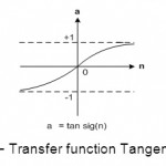 |
Figure 3: Transfer function Tangent Sigmoid Click here to View figure |
For assessment of water quality, we applied the MLP model using average monthly data. According to the Universal Approximator, each multi-layer Perceptron of the ANN with a sigmoid hidden layer and a linear output layer is able to predict each complicated function if the number of neurons is selected precisely (Cybenko, 1989; Hornik, 1991, 1993; Leshno et 1993). This theory decreases the number of hidden layers to the least and decreases the complexity of the network. According to the mentioned theory, all models applied in this research are the MLP with a hidden layer, tangent sigmoid transfer function and linear layer outputs. Figure 4 illustrates the MLP neural network schematic.
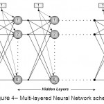 |
Figure 4: Multi-layered Neural Network schematic Click here to View figure |
For calculation of the amount of error in predicting the desired parameter and performance evaluation of models, we used R2 and Root Mean Squared Error (RMSE), as shown in Equations 7 and 8 (Kennedy and Neville, 1964).


Where Xi, Yi, X and Y = the measured data, predicted data, the average of measured data and the mean of predicted data, respectively (Preis et al, 2008; Singh, 2009). The statistical summary of the data is shown in Table 1.
Learning Rate
There is a parameter called the learning rate in the training algorithm of back propagation, which is on the basis of the steepest descent. Its objective is to minimize the sum square error of outputs. The learning rate is indicated by a symbol α and determines the velocity of convergence in this algorithm. The performance of the steepest descent algorithm is enhanced if the learning rate is allowed to alter during the training process.
Maier and Dandy (2000), in a review , studied Neural networks for the prediction and forecasting of water resource variables. They stated that in a review of 43 papers dealing with the use of neural network models for the prediction and forecasting of water resources variables are undertaken in terms of the modeling process adopted and at the vast majority of these networks was trained using the back propagation algorithm.
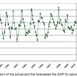 |
Figure 5: Comparison of the actual and the forecasted the SAR for period 1998-2010 Click here to View figure |
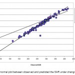 |
Figure 6:The normal plot between observed and predicted the SAR under changing pH Click here to View figure |
Results and Discussion
The MLP model was used for the twelve years monthly (period 1998-2010) data of the Chalgazi River which was collected by Water Authorities of Kurdistan province, Iran. As mentioned previously, according to the universal approximator number of hidden layer decrease to a hidden layer. The rate of the network efficiency depends on applying the appropriate number of neural in the hidden layer. Table 1 indicates a statistical summary of the data that was used in this study. The input layer of the model consisted of eight parameters, including the amounts of sodium, magnesium, calcium, sulfate, chloride, bicarbonate, pH and discharge, which were applied simultaneously, and the output was the SAR. 70% of the data was used for training, 5% for validation and 25% was used for testing of the model. Because of the importance of training most of data should be used as training data. The RSME errors while it used a different number of neurons in a hidden layer for training, testing and total, as shown in Tables 2.
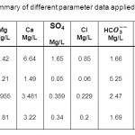 |
Table 1: A statistical summary of different parameter data applied in this study Click here to View table |
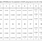 |
Table 2: The rate of RMSE error for prediction of SAR using neuron 2 to 20 in the hidden layer Click here to View table |
Table 2 shows the result of using a different number of neurons in the hidden layer while sodium, magnesium, calcium, sulfate, chloride, bicarbonate, pH and discharge were used as inputs simultaneously, and the SAR was an output of the network. As shown in the both tables, the minimum rate of RMSE occurred while we applied three neurons in a hidden layer. Figure 6 shows the actual and the forecasted SAR. Considering the figure, there is good conformity between the actual and the predicted data, and the correlation coefficient was R2 = 0. 9757. Hence, the developed model may apply for the SAR prediction in water quality management. Comparing the results of this study with the work of Musavi-Jahromi and Golabi (2008) in Karoon River, Iran, there are similarities and agreement between the two results, which confirm the suitability of the ANN model to predict the SAR in river water quality. The differences between the two works are: (1) we gave evidence for using a hidden layer and clearly mentioned type of the model which we applied, and (2) it was evaluated which of the input parameters were significant to forecast the SAR by use of sensitivity analysis. They worked for several water quality monitoring stations, yet in the Chalghazi River there are not as many monitoring stations.
Katoozian et al. (2011) applied the ANN model to Chalghazy and Ghashlagh River water quality parameters using data in the period 1989-2003. The input parameters, which they applied, included EC, discharge, pH and rainfall of two mentioned stations, and they predicted the SAR. The maximum correlation coefficient between predicted and actual SAR was 0.8113. They did not carry out sensitivity analysis. The main advantage and differences between this study and the work of Katoozian et al. (2011) are:
- Data for this study belonged to the period 1998-2009,
- The input parameters to the MLP were rate of flow, pH , Ca, Na, SO4, bicarbonate, chloride and magnesium
- The correlation coefficient between prediction and actual SAR was 0.9757, and the minimum RMSE in training, testing and total were 0.0113, 0.0242 and 0.0175, respectively, in three neurons in the hidden layer.
- Sensitivity analysis was done in this work, which was not done at work of Katoozian et al. (2011)
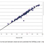 |
Figure 7: The normal plot between observed and predicted the SAR under changing Ca+2 Click here to View figure |
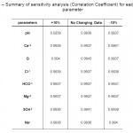 |
Table 3: Summary of sensitivity analysis (Correlation Coefficient) for each input parameter Click here to View table |
Sensitivity Analysis
to assess the effect of each input parameter to the result of the SAR prediction, we increased or declined 10% of one of the input parameters while the other was kept unchanged; then the role of variation of each parameter in prediction of the SAR was identified. We drew the normal plot between the observed and the predicted data for the SAR after changing each input parameter. Figures 6 and 7 indicate the results of the normal plot between the observed and the predicted SAR while each input parameter was changed 10%. The prediction of the SAR was affected only by two of the parameters including pH and Ca, while the other parameters’ effects were not considerable. As indicated in Figure 6, the correlation coefficient for altering pH is 0.0239. This means that the pH has a significant affect on the SAR prediction, however, the discharge, sodium, magnesium, sulfate, chloride; bicarbonate did not affect the prediction noticeably. It may show that the role of the discharge to the SAR perfection is not vital. Figure 7 shows the normal plot for the variation of calcium, as shown in the figure, R2 =0. 92, which means that the calcium has an effect on the SAR prediction; however, the effects are less than the pH variation. Summary of the sensitivity analysis for each input parameter are summarized in Table 3.
Conclusion
Taking into consideration the results and discussions of the applied MLP networks with different neural combinations, the following conclusions can be made:
- The MLP network is adequate for estimation of the SAR prediction, and its accuracy is precise and applicable.
- The minimum RSME error during training, testing and total was 0.01 when applying the MLP network using 3 neural in the hidden layer.
- The correlation coefficient between actual and predicted data is 0.9757, which may show the model’s prediction accuracy.
- The results of sensitivity analysis show pH and calcium parameters are sensitive for prediction of the SAR.
- The outcomes and model may be applicable for water quality management for planning of agricultural water usage.
References
- Asadollahfardi G. Khodadadi A. and Gharayloo R (2010) The assessment of effective factors on Anzali wetland pollution using artificial neural network. Asian j 7 (2): 23-30.
- Asadollahfardi G. and Asadollahfardi R. (2011) The usage of polluted water for agriculture. ISSN: 976-3-8465-1196-1, Lambert academic publishing, Germany.
- Asadollahfardi G. Taklify A. and Ghanbari A (2012) Application of Artificial Neural Network to predict TDS in Talkheh Rud River. Journal of Irrigation and Drainage Egngeering, 363-370, DOI:10.1061 (ASCE) IR, 1943-4774.0000402.
- Ayers R.S.and Tanji K. K. (1981) Agronomic aspects of crop irrigation with wastewater , Pro. water Forum 81,1, ASCE, New York N.Y.pp 579-586.
- Bouwer H. and Idelovitch E. (1987) quality requirement for irrigation with sewer water, j. Irrigation. Drainage. Engineering , 113 (4), 516-535.
- Bouwer H.(1976) Wastewater reuse in arid area water reuse,E.J.Middlebrook,ed,Ann Arbor science publisher, Inc.Ann Arbor, Mich. , pp 137-180.
- Cybenko G. (1989) Approximation by superposition of a sigmoid function. Math Control signals system j, 2, 303-314.
- Coppola E. Poulton M. Charles E. Dustman J. and Szidarovsky F. (2003) Application of artificial neural networks to complex ground water management problems. Natural resources research j, 12 (4), 303-320.
- Dogan E. Sengorur B. (2009) Modelling biological oxygen demand of the Melen River in Turkey using an artificial neural network. Journal of environmental management, 90 (2), 1229-1235.
- Hooshmand Zadeh A. (1995) Geology of Iran bibliography of geology literature in Iran. Iran geological organization publisher, Iran.
- Hornik K.M , Stinchocombe M. and White H. (1989) Multilayer feed forward networks are universal approximators. Neural Network j, 2 (5), 359-366.
- Hornik K.M (1991) Approximation capability of multilayer feed forward networks. Neural network J, 4 (2), 251-259.
- Hornik K.M. (1993) Some new results on neural networks approximation neural networks. Neural network J, 6 (8), 1069-1072.
- Huang W. Foo S. (1997) Neural network modelling of salinity variation in the Apalachicola River. Water research j, 36 (1) , 356-362.
- Islamic Republic of Iran Meteorological Organization (1983) Climate statistic, Http: //www.irimo.ir/ May 18, 2012.
- Kennedy J.B. and Neville A.D. (1964) Basic statistical methods for engineers and scientists. Harper International Edition, New York bases bireme Br, Id 158055.
- Kanani S. Asadollahfardi G. and Ghanbari A. (2008) Application of artificial neural network to predict total dissolved solid in the Achechay River basin. World applied sciences J, 4 (5), 646-654.
- Katoozian S. Kashafi-Desfooli S.M. and Sanadaj Y.S. (2011) Using artificial neural network modeling for SAR and water quality prediction, Ghashlagh parameter (case study, Sanandaj River), A third conference for Urban development, Iran (in Farsi).
- Keiner L. E and Yan X.H (1998) A Neural Network Model for Estimating Sea Surface Chlorophyll and Sediments from Thematic Mapper Imagery Remote Sensing of Environment J, 66, 2,153–165.
- Leshno M, Lin V.Y, Pinkus A and Schocken S (1993) Multilayer feed forward networks with a nonpolynomial activation function can approximate any function, Neural network J, 6, 861-867.
- Maier H.R. and Dandy G.C. (1996) The use of artificial neural networks for the prediction of water quality parameters Water Resources j 32 (4), 1013-1022.
- Maier H.R. and Dandy G.C. (2000) Neural networks for the prediction and forecasting of water resources variables: a review of modelling issues and applications, Environmental Modelling & Software J, 15,1, 101–124
- Maier H.R. and Dandy G.C. (2002). Determining inputs for neural network models of multivariate time series. Microcomputer-Aided civil and infrastructure engineering j, 12 (5) , 353-368.
- Menhaj M.B. (1998) Artificial neural network basis. Amir Kabir University, Vol. 1, Tehran, Iran.
- Menhaj M.B. and Seifipour N. (1998) Application of artificial intelligence in control Professor Hesabi publications, part. 2, Tehran, Iran.
- Musavi-Jahromi S.H. and Golabi M. (2008) Application of artificial neural network in the river water quality modelling. Karoon River, Iran, Journal of applied science, 8 (12), 2324-2328.
- Misaghi F. and Mohammadi K. (2003) Estimating water quality changes in Zayandeh Rud River using an artificial neural network model. Written for presentation at the Canadian society for engineering in agricultural and biological system.
- Mohammadi Y. and Fathi P. (2004) Estimation of average monthly discharge using artificial neural network. A case study: Ghashlagh Dam. Resources journal of agricultural sciences and natural, 15 (4), 258-270 (Farsi language).
- Olyaie1 E. Banejad H. Samadi M.T. Rahmani A.R and Saghi M.H (2010) Performance Evaluation of artificial neural networks for predicting rivers water quality parameter (BOD and DO) in the Hamadan Morad Big River, 20 (3), 200-210.
- Preis A. and Ostfeld A. (2008) A Coupled Model Tree-Genetic Algorithm Scheme for Flow and Water Quality Predictions in Watersheds, Journal of Hydrology, 349 (3-4), 364-375.
- Singh KP.Basant A. Malik A. (2009) Artificial Neural Network Modeling Of the River Water Quality. A case study: Journal of Ecological Modelling, 220 (6), 888-895.
- Razavi F. (2006) Rain prediction applying artificial neural network. MS thesis, Amir Kabir University, Tehran, Iran.
- Zhang Q. and Stanely S.J. (1997) Forecasting raw-water quality parameters for the North Saskatchewan River by neural network modelling. Water research J, 31 (9), 2340-2350.
- Zhang Y, Pulliainen J, Koponen S and Hallikainen M. (2002) Application of an empirical neural network to surface water quality estimation in the Gulf of Finland using combined optical data and microwave data, Remote Sensing of Environment J, 81, (2–3), 327–336.


