Hydrological Regionalization in Relation to Accuracy of Maximum Discharge Estimation
Arash Tavakkoli1 * and Seyed Hashem Hosseini2
1
Department of Civil Engineering,
Torbat-e-Jam Branch,
Islamic Azad University,
Torbat-e- Jam,
Iran
2
Department of Natural Resources,
Torbat-e-Jam Branch,
Islamic Azad University,
Torbat-e- Jam,
Iran
http://dx.doi.org/10.12944/CWE.9.3.41
Copy the following to cite this article:
Tavakkoli A, Hosseini S. H. Hydrological Regionalization in Relation to Accuracy of Maximum Discharge Estimation. Curr World Environ 2014;9 (3) DOI:http://dx.doi.org/10.12944/CWE.9.3.41
Copy the following to cite this URL:
Tavakkoli A, Hosseini S. H. Hydrological Regionalization in Relation to Accuracy of Maximum Discharge Estimation. Curr World Environ 2014;9(3). Available from:http://www.cwejournal.org/?p=7366
Download article (pdf) Citation Manager Publish History
Introduction
Regionalization is generally used in hydrology for transferring hydrological information from basins with statistical data to ungauged basins also the developed regional model can be successfully used for the estimation of the flow duration curves at ungauged sites (E.A. Baltas, 2012). Data transfer can be done more efficiently by dividing the region into homogeneous areas. Homogeneity of the different aspects is determined to create hydrologic homogeneous regions in the hydrological events with the same reaction. One of the most important applications of homogeneous regions is the regional flow analysis. To improve the adequacy and accuracy of hydrological statistics from several meteorological stations, the accuracy of the flow estimated model should be increased. Although the proposed regression models for homogeneous areas have a high correlation coefficient, it is not expected that the estimation of the flow using these models is always accurate. This is due to errors committed during regionalization (ICOLD, 1988). Researchers have studied the importance of determining homogeneous regions using flow analysis and its effect on the increase of accuracy of estimates (Davoodi, 1998). Several researchers have stated that the homogenous regions should be delineated based on climatic characteristics, geographical ranges, political boundaries, and height positions (Murphey, D.E., 1977 and Anil Kumar Kar, 2012), etc. On the other hand, other researchers used hydrological response and basin characteristics as a basis for separating homogenous regions (Strupczewski, 2001), etc. In the present study, cluster analysis and factor analysis were performed for the separation and homogenization of homogeneous regions. A statistical model estimates the stream flows parameters, basin variables define the watershed characteristics. If a regionalization method is prosperous, strong relationships between stream flows properties and basin variables can be realized (Shin-Min Chiang, 2002), etc.
Study Area
The study area of Khorasan Razavi basin is conducted in the northeast of Iran. The total basin area is 118,854 km2. The basin location is encompassed the geographical coordinate of 36.2980o N latitude and 59.6058o E latitude. In terms of geology, the area has two separate tectonic units comprising the sedimentary areas of Hezarmasjed - Koppe Dagh, and Binalood. The climate is classified as both arid and semi-arid based on Demarton’s method. Figure (1) shows the location of the study area.
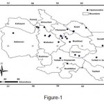 |
Figure 1: Location of hydrometric stations in province of Khorasan Razavi |
Methodology
The approach is according to the research, documentation, analysis and reasoning. Therefore, for the information required is used hydrometric station data. And thence, by using factor analysis are determined the most important factors which used in cluster analysis classification. These regions are classified homogeneous groups. In addition, the data analysis is done by SPSS software.
The methodology consisted of the following major steps:
-
Checking the homogeneity of the entire basin,
-
Selecting prioritized variables,
-
Applying clustering method,
-
Using index flood method for summarizing characteristics
-
Finding the relationship between discharge of return period and physiography, and
-
Selection the regional distribution
Review Statistical Methods
Selection of the most Suitable Regional Frequency Distribution
Subsequent to the testing of data and reconstructing the hydrometric stations, flood frequency analysis was performed during maximum discharge at these stations. This was conducted using the statistical distribution functions including Pearson type II, Pearson log type III, two gamma parameters, three log-normal parameters, and two normal and log parameters using the HYFA software (HYFA is one the statistical software which can be used for statistical analysis, curve fitting and statistical distribution in hydrologic studies).
Table 1: Total variance explained
| Loading Component |
Initial Eigen values | Rotation Sums of Squared | ||||
| Total | Variance Percentage |
Cumulative Percentage |
Total | Variance Percentage |
Cumulative Percentage |
|
| Area | 6.581 | 54.839 | 54.839 | 4.401 | 36.675 | 36.67 |
| Mean annual rainfall | 1.966 | 16.385 | 71.233 | 2.766 | 23.05 | 59.72 |
| Average height | 1.313 | 10.491 | 82.164 | 2.536 | 21.137 | 80.86 |
| Gravilius coefficient | 1.083 | 9.023 | 91.871 | 1.239 | 10.32 | 91.187 |
| 24-hour rainfall | 0.371 | 3.09 | 94.276 | |||
| Net river slope | 0.268 | 2.235 | 96.512 | |||
| River slope | 0.213 | 1.779 | 98.29 | |||
| Basin length | 0.088 | 0.734 | 99.025 | |||
| All waterways length | 0.043 | 0.354 | 99.379 | |||
| The main river length | 0.036 | 0.302 | 99.681 | |||
| Average of basin slope | 0.029 | 0.242 | 99.922 | |||
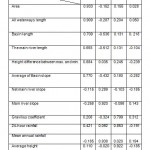 |
Table 2: Varimax rotation matrix Click here to View table |
Factor Analysis and Selection of Independent Variables
As for principal components analysis, factor analysis is a multivariate method used for data reduction purposes. Again, the basic idea is to represent a set of variables of a smaller number of variables. In this case they are called factors. Factor analysis is designed for interval data, although it can also be used for ordinal data (e.g. scores assigned to Likert scales). The variables used in factor analysis should be linearly related to each other. The factor analysis model can be written algebraically as follows. If you have p variables X1, X2, . . . ,Xp measured on a sample of n subjects, then variable i can be written as a linear combination of m factors F1, F2, . . . , Fm where, as explained above m < p. Thus,
Xi=ai1F1+ai2F2+...+aimFm+ei ...(1)
Where the ais are the factor loadings (or scores) for variable i and ei is the part of variable Xi that cannot be ’explained’ by the factors. There are three main steps in a factor analysis:
-
Calculate initial factor loadings.
-
Factor rotation
-
Calculation of factor scores.
In some statistical packages (e.g. SPSS) this choice is actually made at the outset. The second method, choosing eigenvalues over 1, is probably the most common one. The final factor scores are usually calculated using a regression-based approach (Manly, B.F.J., 2005).
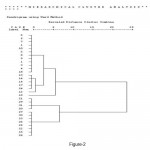 |
Figure 2: Result of hierarchical clustering by using four variables (dendogram) Click here to View Figure |
Cluster Analysis Approach
Cluster analysis was already being used for homogeneous regions by DeCoursey (1973), DeCoursey and Deal (1974), Mosely (1981), Acreman and Sinelair (1986), Burn (1989), Lim and Lye (2003) also Shin-Min Chiang and etc. (2002), Chavoshi and Soleimani (2009), Anil Kumar Kar (2012). DeCoursey (1973) and DeCoursey-Deal (1974) have used cluster analysis for determining homogeneous regions. This method is also known as Decoursey modified method (Wiltshire, S.E, 1986). Cluster analysis searches for and organizes information to determine groups of factors. Some aspects of the factors within each group are similar to each other and do not have dissimilarity with the factors in other groups. If the areas have very similar quantitative properties, these areas will be considered as ‘n’ dimensional spaces which are very close to each other. The similarities of these areas were investigated to measure the distance between them. The method provides a certain measurement known as coefficient of closeness or similarity. Based on this coefficient, similarities between the two areas can be summarized (Tasker, G.D, 1982). Cluster analysis includes the following steps:
-
Selection of the measure of similarity (in the present study, the factor analysis method was used);
-
Standardization of data, which is performed so that all parameters will have the same units;
-
Determination of the Euclidean distance between parameters; and
-
Select a method to determine categories (here is applied cluster analysis with using cumulative class for determining the homogeneous areas).
Table. 3: Discharge median dimensionless quantities for homogeneous regions and whole region
| Q100/Q2 | Q50/Q2 | Q25/Q2 | Q10/Q2 | Q5/Q2 | Q2/Q2 | Region |
| 3.538 | 3.139 | 2.753 | 2.212 | 1.714 | 1 | Homogeneous region (I) |
| 3.793 | 3.341 | 2.888 | 2.271 | 1.776 | 1 | Homogeneous region (II) |
| 3.538 | 3.139 | 2.573 | 2.212 | 1.714 | 1 | Whole region |
Note: Qn is n-years return period discharge
Table. 4: Index flood model in whole region and homogeneous regions
| Region | Model | R2 | SE |
| Whole | Q2 = 64.86 + 0.1632 A | 0.796 | 0.24 |
| Homogeneous (I) | Q2 = 33.17 + 0.1681 A | 0.801 | 0.22 |
| Homogeneous (II) | Q2 = 178.34 + 0.1371 A | 0.94 | 0.182 |
Note: Q2 is the two-years return period discharge (m3/s) and A is the region area (km2)
Table. 5: Multivariable regression models of maximum instantaneous discharge for whole region
| R2 | SE | Model | Return period (year) | ||
| 0.88 | 0.17 | Q2 = 480.9 + 0.154A - 0.151 H | 2 | ||
| 0.88 | 0.18 | Q5975.884A - 0.321 H | 5 | ||
| 0.87 | 0.2 | Q10= 1303.45 +0.38 A - 0.439 | 10 | ||
| 0.86 | 0.19 | Q25= 1725.9 + 0.51 A - 0.594 | 25 | ||
| 0.8 | 0.2 | Q502048.614A - 0.716 H | 50 | ||
| 0.73 | 0.21 | Q100 = 2237 + 0.722 A - 0.841 | 100 | ||
Note: Qn is the maximum instantaneous discharge of n-year return period (m3/s), A is the region area and H is the average height of area (m)
Index Flood Method
Flood index method for regional flood analysis was used for summarizing regional characteristics. Before implementing flood index method, homogeneous areas were specified.
Before applying the index flood method, we must identify the homogenous areas, after that the subscriber base period shall be subjected to the most statistical period. The duration of the selection and reconstruction of subscriber base stations incomplete statistics, the frequency curve is prepared for all stations in the homogeneous region. Finally, the homogeneity test performed and then different return time discharge values are divided by the average annual of return discharge. The ratios obtained for all stations were collected and the above median ratios for each return period were determined. Based on the median ratio for each return period, the regional frequency curve was plotted. Regression was subsequently performed to obtain regional model between annual mean discharge and watershed area (Telori A., 1996 and Chavoshi S., 1997).
Table. 6: Multivariable regression models of maximum homogenous region instantaneous discharge for first
| R2 | SE | Model | Return period (year) | ||
| 0.87 | 0.17 | Q2 = 1085 + 0.126 A - 0.372 H | 2 | ||
| 0.89 | 0.17 | Q5= 1856+0.216 A - 0.63 H | 5 | ||
| 0.88 | 0.18 | Q10 = 2335 + 0.277 A - 0.79 H | 10 | ||
| 0.86 | 0.19 | Q25= 2915+ 0.355 A - 0.981 H | 25 | ||
| 0.82 | 0.19 | Q50= 3335+ 0.413 A - 1.12 H | 50 | ||
| 0.75 | 0.24 | Q100 = 3752 + 0. 47 A - 1.25 H | 100 | ||
Note: Qn is the maximum discharge of n-year return period (m3/s), A is the homogenous region area and H is the average height of area (m)
Multivariate Regression Method
Using this method, the relationship between discharge of different return periods and basin physiographic characteristics is presented instead of plotted basin area-annual mean discharge, (Honarbakhsh, 1993). The General multivariate regression relationship is as follows:
QT=F (Aa, Bb, Cc, .........Zz) ...(3)
Where QT is T- years return period flood; A, B, C,…, Z are parameters that are independent variables of the basin characteristics; a, b, c, …, z is constant values obtained from multivariate regression analysis (Telori A., 1996 and Chavoshi S., 1997).
In the present study, regression equation was formulated for basin characteristics and parameters of probability distribution. After frequency analysis, the appropriate parameters were obtained from each station. Consequently, the regression equations were formed for the estimation of parameters of probability distribution in the important area (Fotouhi A. 2004, and Murphey, D.E., 1977), etc. With the basin characteristics, distribution parameters for different regions without statistics or limited statistics were obtained. Therefore, Qt was computed by the obtained distribution.
Results and Discussion
The study aim is develop a regional model in order to describe the physiographic variation characteristics of parameters and selected model in hydrological homogenous areas. Also, to make a homogenous region model that leads to more accurate estimate of the maximum annual discharge of return varies with period.
Variance Analysis
In the current study, factor analysis was conducted on 17 variables which were measured in the selected areas using the SPSS software. These variables include various characteristics of the basin such as area, perimeter, average slope, master stream slope, average level, average rainfall, maximum 24-hour precipitation, drainage density, Gravilious coefficient, Horton coefficient, Miller coefficient, maximum level, and minimum level. Each unit of measure is different from the other variables. Therefore, all of the units were standardized for accurate comparison of variables. Preliminary results of factor analysis were complex and did not provide the best solution. To maximize the variance of each factor, the factor axes were rotated with varimax rotation until operation results became an independent factor. Identification of the factors was done based on rotated factor loadings. Using the regression estimate method, station factor score matrix was obtained. To limit the number of factors, Kaiser-Meyer-Oklin (KMO) measure of sampling adequacy, which determines the proportion rate of the number of factors selected was performed. Removal of unnecessary variables was based on the anti-image correlation matrix. To measure the discrimination for these variables, which are correlation matrix diagonal elements, the measure of sampling adequacy (MSA) was utilized. In this method, variables with the lowest MSA value are eliminated by considering the significance level of correlation coefficient matrix among variables. In eliminating variables, KMO statistics and variance percentage should be considered. The elimination of a variable will probably increase or decrease KMO value and percentage of variance (Fotouhi A., 2004). After selecting the required variables, factor analysis was conducted. Necessary variables were selected based on the value of KMO = 0.721. KMO is a statistic which tells whether you have sufficient items for each factor. It should be over 0.7. The Bartlett’s test is used to check that the original variables are sufficiently correlated. This test should come out significant (p < 0.05) — if not, factor analysis will not be appropriate (Rencher A.C., 2002). Subsequently, factor analysis was conducted based on the selected variables. Eigenvalues and percentage of variance factors are shown in Table (1). According to Table (1) extracted factors account for 91% change from the previous variable. As can be seen in the table, the first factor is a greater role in the total variance. This is being satisfied factor analysis of parameters (Anil Kumar K., 2012), etc.
Table. 7: Multivariable regression models of maximum homogenous region instantaneous discharge for first
| R2 | SE | Model | Return period (year) |
| 0.904 | 0.17 | Q2 =217.44 + 0.134 A | 2 |
| 0.89 | 0.18 | Q5 =332 + 0.264 A | 5 |
| 0.908 | 0.17 | Q10 =371.5 + 0.367 A | 10 |
| 0.9 | 0.18 | Q25 = 392.7 + 0.513 A | 25 |
| 0.87 | 0.22 | Q50 = 391.5 + 0.632 A | 50 |
| 0.76 | 0.25 | Q100 = 379 + 0.759 A | 100 |
Note: Qn is the maximum instantaneous discharge of n-year return period (m3/s) and A is the homogenous region area (km2)
Using factor analysis of 48 factors were degrees to 4 groups, that the contribution of each factor as follows: The first factor with eigenvalue 25, itself 59 percent of the variance is calculated and explained. The second factor with eigenvalue 25, is capable of calculating and explained 59% of variance. Third Factor: This factor is 6 with eigenvalue 25 in about 59 percent of variance explained. Fourth factor: with eigenvalue 2, interpret 6% of the variance and has 3 factors.
Once the initial factor loadings have been calculated, the factors are rotated. This is done to find the factors that are easier to interpret. The object of the rotation is to try to ensure that all variables have high loadings only on one factor (Manly B.F.J., 2005). In the other word, varimax rotation is a method in which factor structure provides a simple model by maximizing the variance of a data matrix column. The results of the survey using varimax rotation in this research are reduced the factors to 4 factors. Also, the factors have eagle particular value less than 1, are eliminated because cannot determine the variance. As can be seen in the table, the first factor is a greater role in the total variance. The varimax rotation matrix is illustrated in Table (2).
Cluster Analysis
To define homogeneous regions in the study area, cluster analysis was performed by the stratum-clumping method. The characteristics used to be area parameters, average annual rainfall, average basin height, and river net slope. Hierarchical Clustering method with a maximum coefficient of similarity equal to 15 was utilized. This resulted in the determination of two homogenous regions. The dendrogram made with the variables is shown in Figure (2). The cluster 1, just as 19 variables and 12 variables remain for cluster 2. The Hierarchical Clustering method defined the desirable demarcation of basin under different variables.
In the present study, the flood index method of two homogenous regions was accomplished as specified by cluster analysis. The discharge median dimensionless quantities for the whole region and homogeneous regions are shown in Table (3). The Development of regional flood frequency formulas requires following two relationships:
- Relationship between (Qt/Qm) and return period T, and
- Relationship between mean annual flood and catchment characteristics.
Consequently, the dimensionless median according to the relevant return periods based on three log-normal distribution parameters were adjusted and other regional frequency curve was plotted. Using this curve, interpolation by dimensionless medians was conducted to specify other return periods. Modeling of two-year flood was done using basin parameters. The final index flood model in the whole region and homogeneous regions is presented in Table (4). Thus, the flood model five–year return period index can be obtained by multiplying the value of the two-year return period with the median value of dimensionless discharge in the five-year return period (Table3).
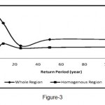 |
Figure 3: Comparison of average values of relative error in the whole region and homogenous regions in the multivariable regression method Click here to View Figure |
Multivariable Regression
When the number of variables selected is large, a small but effective group of variables is considered for further analysis instead of using all the variables. In this regards, multiple regression can be more appropriate for choosing the exact number of variables. The independent variables should again be selected, keeping in view the underlying physical process and a good correlation with the dependent variables. A hydrological regionalization scheme is proposed for the classification of watersheds gauged in this paper. In order to estimate stream flows as ungauged sites, a regression equation such as (Shin-Min Chiang, 2002), etc.
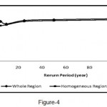 |
Figure 4: Comparison of average values of relative error in the whole region and homogenous regions in the flood index method
Click here to View Figure |
Models to estimate the maximum instantaneous discharge with return periods of 2, 5, 10, 25, 50, and100 years for whole region are shown in Table (5) while those in the homogenous regions are shown in Tables (6) and (7).
Determination of homogeneous regions using the cluster analysis method is the first step in regional flood analysis. Ouarda (2001) determined the characteristics of the study areas, including length of main channel, main channel slope, and mean annual rainfall. Furthermore, Honarbakhsh (1993) stated that the most important parameters affecting flood are the following physiographic characteristics: area, average height, average basin slope, annual rainfall, and length of basin based on the regional analysis of flood. Among the input variables, four factors, namely, area, mean annual rainfall, average basin height, and ground slope of the main river were identified as important factors in homogenizing using the first factor analysis method. These four factors achieved 91.18 percentages of variance. In the next step, basin homogeneity was evaluated by cluster analysis and two homogeneous areas were determined. Based on the four main variables, two types of model were presented: one for the whole region and another for the homogeneous region. Homogenous regions obtained a higher coefficient of determination and less standard error than the overall models. These regions also showed a higher return period R2 and SE values. Furthermore, the relative error of each model in homogenous regions and the whole region was investigated. Figures (3) and (4) present the average relative error determined by multivariate regression and flood index methods in the whole region and homogeneous regions, respectively.
Several studies have been conducted which focused on the importance of hydrological homogeneous regions in increasing the performance and precision of regional analysis models. In the present study, the importance and necessity of creating homogeneous regions were found to be quite evident compared with the overall regional models. Generally, homogenizing results in increased effect of different variables in basins. Consequently, the accuracy of the models will be higher. However, homogenizing can lead to the decrease in the values of the variables probably due to the increased data dispersion. Based on Tables (4), (5), (6), and (7), the SE value in the whole region was greater than the value in the homogeneous regions and R2 value was less than the SE value In addition, homogeneous region models were more efficient than the overall models. Therefore, the relative error in homogeneous regions was less compared with that in the whole region based on the comparison between the relative error in the multivariate regression (Figure 3) and flood index (Figure 4) models with data of the control stations.
Conclusion
The study describes the division of the Khorasan Razavi basin into two homogeneous clusters for making flood frequency .The study also displays how the prioritized variables influence the clustering process. Reducing the dimensionality of variables by using 4 variables out of 17 variables has not had any significant impaction on homogeneity and cluster formation. Regionalization is often done in transferring hydrological data to basins without statistical data. By dividing the region into homogeneous area, the data transferring can be done more efficiently (for region has the same response unto hydrological events). Also in the present study is shown that regression models for homogeneous areas have high correction coefficient, although this model is not always accurate. Consequently, in the research work is carried out that homogeneous areas have the coefficient of determination greater and standard error less than in comparison with wholes models, thus the model accuracy can be increased.
References
- Acreman, M.C., and Sinclair, C.D., Classification of drainage basins according to their physical characteristics: An application for flood frequency analysis in Scotland, J. Hydrol. (Amsterdam), 84 (3–4); 365–380, (1986).
- Anil Kumar Kar, N. K. Goel , A.K. Lohani and G.P. Roy, Application of clustering techniques using prioritized variables in regional flood frequency analysis- case study of Mahanadi basin, Journal of Hydrologic Engineering (ASCE), 17; 213-223, (2012).
- Baltas, E.A., Development of regional model for hydropower potential in western Greece, Global NEST Journal, 14; 4, 442-449, (2012)
- Burn, D.H., Cluster analysis as applied to regional flood frequency, J. Water Resour. Plann. Manage., 115 (5); 567–582, (1989).
- Chavoshi Sattar, Regionalized to instantaneous maximum discharge in arid and semi arid areas, M.Sc. thesis, Department of Civil Engineering, Isfahan University of Technology, (1997).
- Davoodi Rad Ali Akbar, Surveying relationships between morphometric factors and discharge of flood in Iran central basin, M.Sc. thesis, Department of Civil Engineering, Tehran University, (1998).
- DeCoursey, D.G., Objective regionalization of peak flow rates, in flood and droughts, Proc., 2nd Int. Symp. in Hydrology , E. F. Koelzer and K. Mahmood, eds., Water Resources Publications, Fort Collins, CO, 395–405, (1973).
- Decoursey, D.G. and Deal, R.B., General aspects of multivariate analysis with application to some problems in hydrology. Proc., Symp. On Statistical Hydrology , USDA Agricultural Research Service, Washington, DC, 47–68, (1974).
- Fotouhi Akbar and Fariba Asghari, Statistical Analysis by SPSS Software, first edition, Science Publishing Tehran Press, (2004).
- Honarbakhsh Afshin, Regional analysis of flood in the Namak lake basin, Department of Watershed Management M.Sc. Thesis, Tehran University, (1993).
- ICOLD, Design Floods in Egyptian Dams and Barragesn, 16 the congress, Q63R55, Egypt, (1988).
- Lim, Y.H., and Lye, L.M. (2003), Regional flood estimation for ungauged basins in Sarawak, Malaysia, Hydrol. Sci. J., 48(1); 79–94, (2003).
- Kjeldsen, T.r. and J.C. Smithers, Regional flood frequency analysis in the KwaZulu-Natal provinces, South Africa, using the index-flood method, Journal of Hydrology 255, 194-211, (2002).
- Manly, B.F.J., Multivariate Statistical Methods: A primer, Third edition, Chapman and Hall, (2005).
- Mosley, M . P. , Delineation of New Zealand hydrologic regions, J. Hydrol. (Amsterdam), 49 (1–2); 173–192, (1981).
- Murphey, D.E. and E. Wallance and L.J. Lane, Geomorphic parameters predict hydrograph characteristics in the Southwest, Water Resources Bulletin, 13(1); 217-238, (1977).
- Ouarda, B.M.J., C. Girard and B. Bobee, Regional flood frequency estimation with canonical correlation analysis, Journal of Hydrology, 254, 157-173, (2001).
- Rencher, A.C., Methods of Multivariate Analysis, Second edition, Wiley, (2002).
- Rezaei Abdulmajid, Introduction to Applied Regression Analysis, first edition, Isfahan University of Technology press, (1997).
- Shin-Min Chiang, Ting-Kuei Tsay and Stephan J. Nix, Hydrologic regionalization of watersheds, I: Methodology Development, Journal of Water Resources Planning and Management (ASCE), 128; 1 (3), 3-11, (2002).
- Strupczewski, W.G. and Z. Kaczmarck, Non-stationary approaches to at-side flood frequency modeling ²² Weighted least squares estimation, Journal of Hydrology, 248; 143-151, (2001).
- Tasker, G.D., Comparing methods of hydrologic regionalization, Water Resources Bulletin, 18(6); 965-970, (1982).
- Telori Abdulrasoul, Effective factors in the occurrence or exacerbation of flood, proceedings of specialized flood rivers, Iran’s Hydraulic Association (1996).
- Wiltshire, S.E., Regional flood frequency analysis ÉÉ: Homogeneity statistical, Hydrological Sciences Journal, 31(3); 321-333, (1986).


