Current World Environment

Introduction

Streamflow forecasting is a key component in sustained development and based on environmental issues. It has been an important subject for the researchers from the middle of the 20th century. Different approaches such as regression (Sun et al. 2014; Rehman and Saleem, 2014, Dehghani et al. 2014), conceptual (Jain and Srinivasulu, 2006; Xu et al. 1996) and intelligent(He et al. 2014; Liu et al. 2014; Sudheer et al. 2014) models are used for stream flow forecasting. Artificial intelligence models, especially Artificial Neural Networks (ANNs) have been applied for stream flow forecasting in several researches. Artificial Neural Network (ANN) is a nonlinear black-box statistical approach (Kalteh, 2013). ANN s are suitable for dealing with the intrinsic characteristics commonly present in hydro logical processes (Fajardo Toro, 2013). ANN is appropriate for the problems which the input is high dimensional, data are possibly noisy and not important to know the weights. Literatures in the last two decades show a high interest in using ANN for hydro logical processes, forecasting and different ANN architectures were used for this purpose. Most studies have been done by feed forward error back propagation(Karunanithi et al., 1994; Kisi, 2004). The standard back propagation algorithm (SBPA) has some problems including very low speed training convergence and easy entrapment in a local minimum (Haykin, 1999). The Levenberg-Marquite algorithm proposed as a training function to overcome these problems.

One of the problems in ANN planning is presence of the complex structures which lead to networks with heavy architecture. In this regard, Coulibaly et al. (2000) utilized Stop Training Algorithm (STA) to solve this problem. It is possible to find several effective factors which cause networks with simple architecture. Input selection is a crucial step in ANN implementation. The lack of pertinent input impairs the network application to map the input into a close estimate of the observed stream flow. If the number of weights in ANNs is more than of samples in the training of ANNs to some extent, “over fitting” may be caused (Haykin, 1999). In the case of a high number of input variables, the probability of correlation between the input variables increase and ANN hardly can find the optimized models. Therefore, if possible, it recommends reducing input variables even though this causes some of the information omitted. Principal Component Analysis (PCA) is a proper method for data reduction (Dehghani et al. 2014; Noori et al. 2011). PCA has been used widely in different environmental issues.

Forecasting is associated with uncertainty. It means that the forecasted values will not be happen exactly all the time and they oscillate around the predicted values. So investigating the uncertainty associated with the forecasted values is an important issue in environmental processes forecasting. Different methods were used for uncertainty analysis in the past decades (Dehghani et al. 2014; Zhao et al. 2011; Viola et al. 2009). Monte Carlo simulation is one of the most popular methods in uncertainty analysis. Uncertainty analysis and assigning confidence intervals enable the water resources decision makers to have a better understanding of water resources in early future and make decisions based on this information.

In this paper by considering the above explanation,monthly stream flow forecasted via ANN. Also the Monte Carlo simulation method is used to investigate the uncertainty of forecasted values. In sections 2 and 3, the study area and methodology are described, respectively. Model performance and discussions are presented in section 4 and the conclusions are drawn in section 5.

Study area and data

The Great Karun Basin is located in southwest of Iran (Fig. 1). The basin covers an area of 67112 km² at the mouth of the Persian Gulf. This basin produces over 25% of total surface water resources in Iran and significantly affects the agricultural, social and environmental aspects of human life in this region.

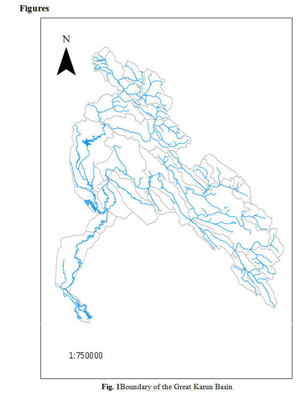Figure 1: Boundary of the Great Karun Basin Click here to View Figure

Based on the high surface water potential in the basin that supplies water to various users and generates hydro power, hydro logic studies and stream flow forecasting are vital to efficient water planning and management. This study focuses on Dez River sub basin within the Great Karun. Fig. 2 shows the study area and the hydro metric station network in the selected area. The reason for selecting the tributaries of the Dez network was because the data at some downstream stations may have been affected by upstream water withdrawals.  However, water use is negligible in the tributary rivers. As a result, part of the Dez river system up to the Sepiddasht hydro metric station was designated as the study area.

Figure 2: Boundary of the study area and location of hydrometric stations Click here to View Figure

A total of seven hydro metric stations were studied in this research. Referring to Fig. 2, the stations are Rahimabad, Dorudtire, Sepiddasht, Chamchit, Moruk, Daretakht and Dorudmarbere. All the stations have data from 1955 to 2009 for a total of 648 months stream flow data. Table 1 represents the monthly stream flow statistics for all hydro metric stations. The flow coefficient of variation oscillates between 1 and 1.95. This is a typical characteristic of stream flow in basins of Mediterranean climate that makes the forecast a challenging task.

Table 1: Monthly stream flow statistics at studied hydro metric stations

Statistics	Rahimabad	Moruk	Dorodtire	Daretakht	Dorodmarbere	Chamchit	Sepiddasht
Max (CMS)	41.86	53.70	156.89	82.16	197.17	76.57	123.68
Min (CMS)	0.01	0.00	0.37	0.00	0.74	1.05	2.00
Mean (CMS)	5.37	4.39	15.45	3.45	9.21	7.34	18.60
standard deviation (CMS)	5.38	6.92	19.86	6.72	13.07	7.50	19.26
coefficient of variation	1.00	1.58	1.28	1.95	1.42	1.02	1.04

Methodology

Artificial neural networks        

ANN customary architecture is composed of three layers of neurons: input layer, hidden layer and output layer (Haykin, 1999). A neuron response is based on the weighted sum of all its inputs according to an activation function. A feed-forward network was adopted for this study since feed-forward ANN has been shown to have a computational superiority in comparison to other paradigms (Hornik et al., 1989). The network was trained by the back-propagation algorithm through the split-validation procedure. Available data was divided into three sets: a training set, a validation set, and a test set. The training set is used to fit ANN model weights, the validation to select the model variant that provides the best level of generalization, and the test set is used to evaluate the chosen model against the remaining data. The number of neurons between 2 to 6 was chosen by trial and error. All input and output variables were standardized to [0.1, 0.9] scale as follows (Rajurkar et al., 2004):




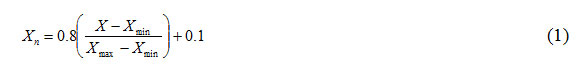
where X is input variable, X_min and X_max are the minimum and maximum values of input variable and X_n is the standard value.

The total number of weights to be determined in a neural network is, (N_inp ⁺¹) ^{x hid + (N_hid +1) x1} for one hidden layer. This essentially accounts for all the connections between neurons in the layers. The number of neurons in the hidden layers increases the amounts of connections and weights to be fitted. This number cannot be increased without limit because one may reach a situation where the number of the connections to be fitted is larger than the number of the data pairs available for training. Although the neural network can still be trained, the case is mathematically undetermined. Mathematically, it is not possible to determine more fitting parameters than the available data points.

In this study a model based on a feed forward neural network with a single hidden layer is used. The back propagation (BP) algorithm is used to train the network. The BP algorithm is essentially a gradient descent technique that minimizes the network error function (Haykin, 1999).

Principal Component Analysis

Principal Component Analysis (PCA) is a method to identify the pattern in the data. This is a powerful tool to reduce the high dimensionality of data, especially when the data sets are highly correlated. Input variables are changed into PCs that are independent i.e. the information of input variables are presented with minimum losses in PCs (Helena et al., 2000; Noori et al., 2011). PCs specified by the equation below.



Where Z_i represents PCs, a_i is related eigen vector and X_i are also input variables. This information achieved by solving equation (3) (Johanson and Wichern,1982).

|R - I λ | = 0         (3)

Where, I is unit matrix, R is variance-covariance matrix and  is eigen value. By these eigen values, we can achieve the eigen vectors. . Details of the method are presented by, for example, Camdevyren et al. (2005), Noori et al. (2011), Helena et al. (2000), Dehghani et al. (2014).

Model evaluation

As there is no single evaluation criterion, it is important to apply a multi-criteria assessment of ANN skill (Dawson et al., 2002; Kumar et al., 2005). Dawson et al. (2007) summarized some evaluation statistics and they may be calculated by Hydrotest, a web-based toolbox, on hydrotest website (http://www.hydrotest.org.uk). We applied 12 criteria to evaluate the model performance.

Uncertainty analysis

In order to determine the uncertainty in Stream flow forecast, ANN modeling procedure was implemented in a Monte-Carlo framework as introduced by Marce et al. (2004). Monte-Carlo simulation involves repeated generation of random parameters from their probability distributions, and then computing the statistics of the output. In this research Bootstrapping was used for resampling. The input database randomly re sampled without replacement 1000 times, maintaining the ratio between the calibration (training and validation) and test sets. The 95% confidence interval of estimation is reported here due to the fact that this confidence interval provides more information than other statistical values about the range of predictions associated with the model (Noori et al., 2010c) The 95% confidence intervals are determined by finding the 2.5th and 97.5th percentiles of the constructed distribution (Noori et al., 2009).

Results and Discussion

For Stream flow forecasting, three scenarios were considered (table 2). In the first scenario, monthly stream flow forecasted using Rahimabad and Moruk streamflow as input. In the second scenario using all hydro metric stations upstream of Sepiddasht station, the stream flow forecasted in Sepiddasht station.

Table 2: Scenarios and input ariables

Input	Target station	Scenario Number
Rahimabab, Moruk	Dorudtire	1
Rahimabad, Moruk, Dorudtire, Dorudmarbere, Daretakht,Chamchit	Sepiddasht	2
PC	Sepiddasht	3

In the third scenario, PCA was applied to the inputs in the second scenario to reduce the high dimensionality of data. Results indicated that the first PC reproduces 84% of variance of data. So, the first PC was selected as the input in the third scenario.

For ANN modeling, stream flow time series divided into three parts. The last 120 months river discharge assigned for test, 100 months for validation and the rest of the data for training then the model applied to the time series. Figs. 3 to 5 shows the ANN modeling of stream flow in test phase. From these figures it can be obtained that the model had a suitable performance in the test phase especially for Dorudtire station. However the ANN model is underestimating especially in extreme values.  

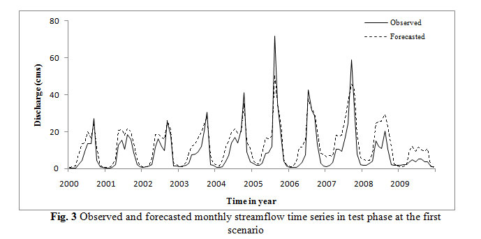Figure 3: Observed and forecasted monthly streamflo time series in test phase at the first scenario Click here to View Figure

 

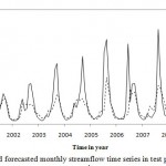Figure 4: Observed and forecasted monthly stream flow time series in test phase at the second scenario Click here to View Figure

 

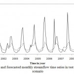Figure 5: Observed and forecasted monthly stream flow time series in test phase at the third scenario Click here to View Figure

 
The mean, minimum and maximum observed values and forecasted values in the test phase are presented in table 3 Results indicated that the model is underestimated in maximum and mean values while in minimum value the model is overestimated.

Table 3: Monthly stream flow statistics of observed and forecasted time series in the test phase

Forecasted			Observed
Mean (cms)	Minimum (cms)	Maximum (cms)	Mean (cms)	Minimum (cms)	Maximum (cms)	Scenario Number
12.88	0.62	50.6	9.27	0.4	71.6	1
15.43	2.81	52.28	19.4	2	106.1	2
16.26	8.63	31.31				3

 
In general the model performed better at Dorudtire station.The model follows the observed time series pattern properly in all scenarios. This is one of the most important factors in time series modeling. For more investigation, 12 statistical criteria are calculated for the test phase (table 4). The bold and italic values show better performance.

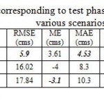Table 4: Statistical criteria corresponding to test phase of monthly streamflow forecast in various scenarios  Click here to View table

The first seven criteria are about modeling error estimation. Based on these criteria the model had the best performance at Dorudtire station.  For a perfect model these seven metrics would be zero. RAE comprises the total absolute error made relative to what the total absolute error would have been if the forecast had simply been the mean of the observed values (Dawson et al. 2007). RAE value is better in the first and second scenarios.The four remaining metrics, including R, IoAd, CE and PI have the best values for first scenario among the other scenarios. Roscillates between 0.67 and 0.92 among different scenarios. However R is insensitive to additive and proportional differences between the observed and model led data sets, so high values can be obtained, even if the modeled values are considerably different from the observed values in terms of magnitude and variability. So for better judgment, Nashe-Sutcliffe coefficient (CE) is used which is sensitive to differences in the observed and modelled means and variances. PI is persistence index and is very similar to CE. IoAd is used to calculate the index of agreement. In overall the model performance is appropriately acceptable in all scenarios.

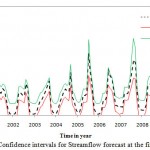
A practical way of quantifying the accuracy of the forecast is by estimating the confidence interval of prediction. The wider the interval, the smaller is the accuracy of the forecast and vice versa. The Monte Carlo simulation was conducted for setting upper and lower confidence bands for stream flow forecasting in different scenarios. Results of 95% confidence intervals are shown in figures 6 to 8.  

Figure 6: Confidence intervals for Stream flow forecast at the first scenario Click here to View Figure

 

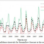Figure 7: Confidence intervals for Stream flow forecast at the second scenario Click here to View Figure

 

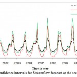Figure 8: Confidence intervals for Stream flow forecast at the second scenario Click here to View Figure

Results indicated that in the first scenario, all forecasted values lie within the confidence intervals. It can be conducted that ANN performed satisfactorily in forecasting monthly stream flow in the first scenario. Also, all the forecasted values in second scenario lie within the confidence intervals while in the third scenario a large number of forecasted values lie out of confidence intervals. 75% of forecasted values in third scenario lie out of confidence intervals which show the model performed poorly in forecasting streanflow. Most of the forecasted values are out of upper bound which shows that the model is not capable to predict the upper band properly.

Conclusion

In this study by using ANN, monthly stream flow was forecasted in three scenarios in Karin basin in Iran. Also uncertainty analysis was conducted to predict the confidence intervals. Results indicated that the model is capable to forecast monthly stream flow satisfactorily although in some cases the model is over/underestimated. However there are some considerations. Base on the statistical criteria the model performed well in the first and second scenarios while the model performance is poor in the third scenario. It can be concluded that the model is sensitive to the quality of input and more information leads to better performance. So by using PCs as input, the model will lose some information and the model performance will be worse than the other scenarios. In reverse, using PC(s) as input decreases the model complexity. The difference between first and second scenarios may due to the water withdrawal upstream of Seppiddasht hydro metric station. Beside the statistical criteria, uncertainty analysis provides a good evaluation of stream flow forecasting. Monte Carlo simulation which is used in this research is a powerful tool for uncertainty analysis and performed well in the confidence interval prediction.

References
 

1. Camdevyren H., Demyr N., Kanik A., Keskyn S. (2005). Use of principal component scores in multiple linear regression models for prediction of Chlorophyll-a in reservoirs. Ecological Modelling, 181: 581–589.
2. Coulibaly P., Anctil F., Bobee B. (2000). Daily reservoir inflow forecasting using artificial neural networks with stopped training approach. J. of hydrology, 230:244-257.
3. Dawson C.W., Wilby R.L., Chen Y. (2002). Evaluation of artificial neural network techniques for flow forecasting in River Yangtze, China. Hydrol. Earth Syst. Sci., 6: 619–626.
4. Dawson CW, Abrahart RJ, See LM (2007) Hydrotest: A web-based toolbox of evaluation metrics for the standardized assessment of hydrological forecasts. Environ. Model. Softw. 22:1034–1052.
5. Dehghani M., Saghafian B., Nasiri Saleh F., Farokhnia A., Noori R. (2014). Uncertainty analysis of streamflow drought forecast using artificial neural networks and Monte-Carlo simulation. Int. j. climatol., 34: 1169–1180.
6. Dehghani M., Saghafian B., Rivaz F., Khodadadi A., (2014). Monthly streamflow forecasting via dynamic spatio-temporal models. Stoch Environ Res Risk Assess., DOI 10.1007/s00477-014-0967-3.
7. Fajardo Toro C.H.,Meire S.G.,Galvez J.F., Fdez-Riverola F. (2013). A hybrid artificial intelligence model for river flow forecasting. Applied Soft Computing 13:3449–3458.
8. Haykin, S., (1999). “Neural Networks: A Comprehensive Foundation.” 2^nd ed., Prentice Hall., New Jersey.
9. He Z., Wen X., Liu H., Du J. (2014). A comparative study of artificial neural network, adaptive neuro fuzzy inference system and support vector machine for forecasting river flow in the semiarid mountain region. J. of Hydrology, 509:379-386.
10. Helena, B., Pardo, R., Vega, M., Barrado, E., Fernandez, JM., Fernandez, L., (2000). Temporal evolution of groundwater composition in an alluvial aquifer (Pisuerga river, Spain) by principal component analysis. Water Research 34: 807-816.
11. Hornik K., Stinchcombe M., White H. (1989). Multilayer feedforward networks are universal approximators. Neural Networks, 2(5): 359-366.
12. Jain, A., Srinivasulu, S. Integrated approach to model decomposed flow hydrograph using artificial neural network and conceptual techniques. Journal of Hydrology 317 (2006) 291–306.
13. Johnson R.A., Wichern D.W. (1982). Applied Multivariate Statistical Analysis,Prentice Hall.
14. Kalteh, A.M. (2013). Monthly river flow forecasting using artificial neural network and support vector regression models coupled with wavelet transform.Computers & Geosciences, 54:1-8.
15. Karunanithi, N., Grenney, W.J., Whitley, D., and Bovee, K. (1994). “Neural networks for river flow prediction.” Journal of Computing in Civil Engineeirng., 8: 201–220.
16. Kisi, O. (2004). “River flow modeling using artificial neural networks.” Journal of Hydrologic Engineering., 9(1), 60–63.
17. Kumar D.N., Raju K.S., Sathish T. (2005). River Flow Forecasting using Recurrent Neural Networks. Wat. Res. Manage., 18:143–161.
18. Liu Z., Zhou P., Chen G., Guo L., (2014). Evaluating a coupled discrete wavelet transform and support vector regression for daily and monthly streamflow forecasting. J. of Hydrology, DOI: 10.1016/j.jhydrol.2014.06.050.
19. Marce R, Comerma M, Garcia JC, Armengol J. (2004). A neuro-fuzzy modeling tool to estimate fluvial nutrient loads in watersheds undertime-varying human impact. Limnology and Oceanography Methods. 2: 342–355.
20. Noori R, Abdoli MA, Farokhnia A, Abbasi M. (2009). Results uncertainty of solid waste generation forecasting by hybrid of wavelettransform-ANFIS and wavelet transform-neural network. Expert Systems with Applications 36(6): 9991–9999.
21. A., Ghafari Gousheh M. (2011). Assessment of input variables determination on the SVM model performance using PCA, Gamma test, and forward selection techniques for monthly stream flow prediction. J. of hydrology, 401:177-189.
22. Rajurkar, M.P., Kothyari, U.C. & Chaube, U.C. (2004) Modeling of the Daily Rainfall-Runoff Relationship with Artificial Neural Network. J. Hydrol., 285, 96-113.
23. Rehman S.U., Saleem K. (2014). Forecasting scheme for swan coastal river streamflow using combined model of IOHLN and Niño4. Asia-Pacific Journal of Atmospheric Sciences, 50(2): 211-219.
24. Sun A.Y., Wang D., Xu X. (2014). Monthly Streamflow Forecasting Using Gaussian Process Regression. J. of hydrology, 511(16): 72-81.
25.  Sudheer C.h., Maheswaran R.,  Panigrahi B.K., Mathur S. (2014). A hybrid SVM-PSO model for forecasting monthly streamflow. Neural Computing and Applications, 24(6):1381-1389.
26. Viola F., Noto, L.V., Cannarozzo, M., La Loggia G. (2009). Daily streamflow prediction with uncertainty in ephemeral catchments using the GLUE methodology. Physics and Chemistry of the Earth, Parts A/B/C, 34(10-12): 701-706.
27. Xu, C.-Y., Seibert, J., Halldin, S., 1996. Regional water balance modelling in the NOPEX area: development and application of monthly water balance model. Journal of Hydrology 180, 211–236.
28. Zhao T., Cai X.,Yang D. (2011). Effect of streamflow forecast uncertainty on real-time reservoir operation. Advances in Water Resources, 34(4): 495–504.