A Comparative Analysis of ARIMA and other Statistical Techniques in Rainfall Forecasting: A Case Study in Kolkata (KMC), West Bengal
Md Juber Alam
*
 and Arijit Majumder
1
Department of Geography,
Jadavpur University, Kolkata,
West Bengal
India
http://dx.doi.org/10.12944/CWE.18.3.37
Copy the following to cite this article:
Alam M. J, Majumder A. A Comparative Analysis of ARIMA and other Statistical Techniques in Rainfall Forecasting: A Case Study in Kolkata (KMC), West Bengal. Curr World Environ 2023;18(3). DOI:http://dx.doi.org/10.12944/CWE.18.3.37
Copy the following to cite this URL:
Alam M. J, Majumder A. A Comparative Analysis of ARIMA and other Statistical Techniques in Rainfall Forecasting: A Case Study in Kolkata (KMC), West Bengal. Curr World Environ 2023;18(3).
Download article (pdf)
Citation Manager
Publish History

Introduction
Rainfall is the primary supply of water for those whose entire existence is reliant on it. Rainfall prediction has become a significant concern in recent years, attracting the attention of government agencies, industries, risk assessment agencies, and the research community. Rainfall prediction models can aid in preserving people's lives and property while indirectly supporting the country's economy. Effectively forecasting long-term rainfall and quantification is essential for water resource planning and management 1–3. Long-term rainfall data prediction in meteorology can aid decision-making processes carried out by organizations responsible for catastrophe square avoidance 4. Rainfall prediction is a challenging endeavor due to the non-linear character of climate processes. In recent years, data-driven (empirical) approaches have surpassed knowledge-driven (physical) approaches in terms of popularity 5. The effective use of several data-driven models in hydrology has opened new dimensions for the usability of deep neural networks for time series analysis. Box and Jenkins proposed the autoregressive integrated moving average model (ARIMA), generally known as the Box–Jenkins model, for time-series forecasting 6. The Autoregressive model, Autoregressive Moving Average (ARMA), and Autoregressive Integrated Moving Average (ARIMA) models have all been used extensively in hydrological forecasting 7-8. ARIMA is an enlarged form of the ARMA model, and it is one of the most effective models with a long history of use 9–11. Sequential modeling was employed to forecast monthly precipitation in India and demonstrate that a deep learning network can be used successfully for time series analysis in the realm of hydrology and related fields 12. A comparative study using machine learning techniques has been used to build models for rainfall prediction 13. A comparative study of various statistical and deep learning techniques were carried out to forecast long-term pollution trends in Kolkata and it was discovered that statistical methods such as auto-regressive (AR), seasonal auto-regressive integrated moving average (SARIMA), and Holt-Winters outperformed the deep learning methods 14. The rainfall intensity of Coonoor in the Nilgiri district of Tamilnadu was predicted using regression techniques and other statistical models. The regression techniques employed for prediction were support vector regression (SVR), Random Forest (RF), and Decision Tree (DT), demonstrating that Random Forest is the best regression strategy for rainfall prediction (RF) 15. A comparison of ANFIS, ARIMA, and the suggested Fuzzy based Curve fitting for weather forecasting was conducted using SSE, R2, RMSE, and MAE, and it was discovered that the curve fitting based on fuzzy logic outperforms ANFIS and ARIMA 16. Statistical downscaling local polynomial regression was used to derive future rainfall estimates in the catchment of the Idukky reservoir in Kerala, India 17. The rainfall in the city of Bengaluru, India, was forecasted using seasonal Naive, triple exponential smoothing and seasonal ARIMA time series models where many scale dependent error predictions methods and inferential analysis were used to assess the accuracy of forecasts from these time series models and the results suggest that the seasonal autoregressive moving average model delivers more accurate results 18. A comparison of 4 different machine learning algorithms (K-Nearest Neighbor, Logistic Regression, Random Forest Classifier, and Support Vector Machine) in solar flare forecasting shows that Logistic Regression and Support Vector Machine algorithms perform exceptionally well in forecasting active region flaring potential 19. Recent studies have utilized non-linear models, including artificial neural networks (ANNs) and classification and regression trees (CART), to predict precipitation in various climate conditions 20–22. Forecasting rainfall directly impacts the security and economic stability in any region, which is typically a complex phenomenon. The Indian cities like Kolkata, one of the country's largest cities, have more than 80 percent built up area 23. Due to huge coverage of the built-up area of Kolkata Municipal Corporation (KMC) the city faces water crisis during non-monsoon periods while it faces urban flood during the monsoon period frequently. Hence, the management of rainwater in a sustainable way should be a major focus of research in this area. Rainwater harvesting may serve as an alternative method to reduce urban floods and, at the same time, maintain the water supply to create favorable conditions to meet the water demand of the city. Therefore, in order to invest for rainwater harvesting or any other sustainable planning to meet the water demand of KMC, rainfall forecasting is of utmost importance. Though many works have been done on rainfall forecasting but there is a lack of studies in comparative analysis of various degree of polynomial curve and ARIMA to find the best fit model in the study area to better forecast the rainfall. Therefore, this study aims to identify the optimal model by evaluating the root mean square error (RMSE) and examining the relationship between the coefficient of determination (r2) and RMSE in identifying the best fit model. The focus of this study is to determine the optimum model for forecasting rainfall using different techniques like the auto-regressive integrated moving average (ARIMA) and other statistical regression techniques. In this study, a comparative analysis of ARIMA and other statistical techniques like a different degree of a polynomials have been used in Rainfall Prediction in Kolkata (KMC), West Bengal. For this purpose, 120 years of monthly and annual rainfall data of IMD (Indian Meteorological Department) from 1901 to 2020 of Kolkata has been retrieved from the Indian water portal “Water Resource Information System” (WRIS) and tries to forecasting rainfall using ARIMA, and different degree of Polynomial regression for identification of the best model.
Materials and Methods
Study Area
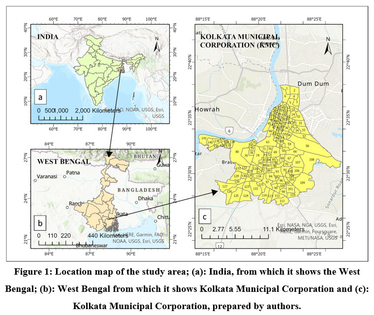
As per the Official website of the Kolkata Municipal Corporation, the current study area is extended between 22°27'28" North to 22°38'20" North, and 88°15'50" East to 88°28'45 " East (Fig. 1). The whole area under study is 187 km2, which has been attained using ArcMap 10.2 by vectorization the Kolkata Municipal Corporation (KMC) map in UTM projection and WGS84 datum. The area under study is bordered on the north and north-east by the district of North 24 Parganas, on the south by the district of South 24 Parganas, and on the west by the Hooghly River. The entire region is located in the Ganges Delta, which is a natural recurrence. According to the Indian Meteorological Department (IMD), the research region exhibits a tropical wet and dry climate. The main seasons are summer, wet autumn, brief winter and summer which is characterized by excessive humidity. The southwest monsoon continues to be the dominant source of precipitation in the study region and the wettest months of the year are June, July, August and September.
 | Figure 1. Location map of the study area; (a): India, from which it shows the West Bengal; (b): West Bengal from which it shows Kolkata Municipal Corporation and (c): Kolkata Municipal Corporation, prepared by authors.
|
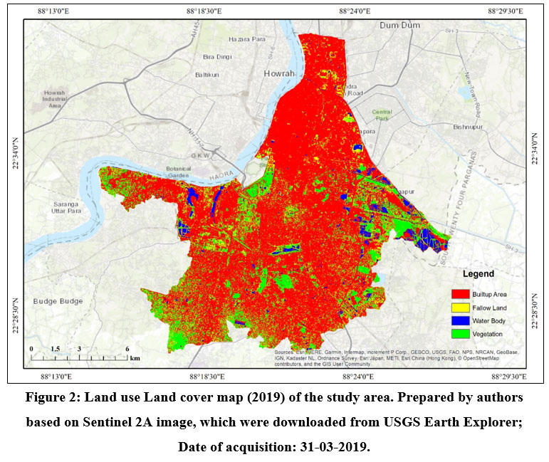
The Kolkata Municipal Corporation's land use and land cover map have been generated using ERDAS IMAGINE 2014 using the Sentinel 2A (2019) image. The overall built-up area (Fig. 2) in KMC has been found to account for 82.23 percent of the total area in 2019. The huge built-up area in KMC combined with a diminishing trend in ground water level raises concerns about the area's long-term water availability. As a result, this study becomes critical for the city's long-term viability.
 | Figure 2: Land use Land cover map (2019) of the study area. Prepared by authors based on Sentinel 2A image, which were downloaded from USGS Earth Explorer; Date of acquisition: 31-03-2019.
|
Database and Methodology
To achieve the aforementioned goal, the model was built using the monthly and annual rainfall data, which has been retrieved from a web-based spatial data portal from India’s water resource information system (https://indiawris.gov.in/wris/#/rainfall) from 1901 to 2020.
Rainfall Forecasting
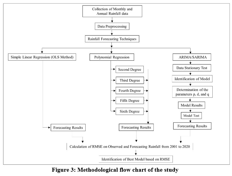
For rainfall forecasting monthly rainfall data have been integrated to produce total rainfall on yearly basis. In this paper, several statistical approaches have been used to study rainfall forecasting, including Autoregressive Integrated Moving Average Method (ARIMA) using python linear (Ordinary Least Square Method) and polynomial regression in MS Excel. Finally, to find the best fit model the Root Mean Square Error (RMSE) has been calculated using observed and forecasted rainfall data from 2001 to 2020. The methodological framework of the study has been shown in Fig. 3 The process of forming assumptions about the future values of investigated variables is known as forecasting 6. The serial correlation effect has been checked since it plays a vital role in assessing and ultimately reducing the uncertainty of rainfall forecasting before it was examined in detail.
 | Figure 3: Methodological flow chart of the study .
|
Augmented Dickey Fuller Test (ADF Test)
Augmented Dickey Fuller Test is one of the most widely used statistical test when it comes to analyzing the stationary of a series. For the prediction of rainfall with ARIMA it is necessary to check the time series data whether the data is stationary or not. In this study to check the data whether it is stationary or not ADF test have been applied using python. For this test, adfuller function have been imported from ‘statsmodels.tsa.stattools’ library in python.
Serial Correlation Effect
The Serial correlation or auto correlation is used to find a link between the variable's current value and any prior values that must be accessed. It's an authentic way to find hidden trends and patterns in time series data that would otherwise go unnoticed. While using ARIMA to forecast rainfall, it has been assumed that the observed time-series data is serially independent. However, significant serial correlation coefficients in time series rainfall data may arise, necessitating the testing of serial correlation effect while reviewing a series of historical data.
The Autocorrelation and partial autocorrelation functions in Python have been used to evaluate the significant autocorrelation coefficients with varying lagged values at a confidence level of 0.05. Lag-1 autocorrelation is often used to examine the influence of serial correlation in time series data. 24. The simple correlation coefficient between the first observation N-1, Xt, t =1,2,3,...,N-1 and the subsequent observations, Xt+1, t = 2,3,...,N-1 is known as the lag-1 autocorrelation coefficient 25. The formula for calculating the relationship between Xt and Xt+1 is given below-
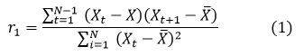
is the total mean.
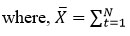
The coefficient r1 is investigated to test its significance. The probability limitations of a two-tailed independent series' correlogram are illustrated below 25.-
where, N denotes the sample size and k denotes the lag.
The data are presumed to be serially dependent if r1 is outside the provided confidence interval and serially independent if r1 falls within the interval.
The Auto-Regressive Integrated Moving Average (ARIMA)
Autoregressive Integrated Moving Average (ARIMA) or Box-Jenkins have been extensively used as forecasting techniques. The autocorrelation function (ACF) and partial autocorrelation function (PACF) of the sample data were proposed as the main tools for determining the ARIMA model's order 6. The model is expressed as ARIMA (p, d, q), where p represents the order of the auto regressive process, d represents the order of the stationary data and q represents the order of the moving average process 26. The ARIMA model is implemented in the following steps 27.-
Identification of Model
When time series data are stationary, the ARIMA model is useful. The first step is to determine whether the time series data is stationary or not before proceeding any further. Before forecasting with ARIMA, it is necessary to make a time series stationary if it has a trend or seasonality component.
Identification of PACF and ACF parameters
In order to use the ARIMA model, it is necessary first to identify the value of d (stationary data), the number of residual lag values (q) and the dependent lag value (p). The key tools for detecting q and p, as well as correlation are ACF (autocorrelation function) and PACF (partial auto correlation function) which displays the plot of ACF and PACF values for lag. The partial autocorrelation coefficient measures the similarity between Xt and Xt-k whereas the lab effect times 1, 2, 3,..., k-1 are taken as constant
Build the optimal ARIMA Model
There can be different ARIMA models based on the outcomes of the stationary detection and the determination of ACF and PACF. Hence, the auto-regressive parameters are determined. To identify the best order of the model in this analysis the auto_ARIMA function has been used which automatically gives the optimum order for this model. In Python, the auto_ARIMA function finds the best order for the model's parameters by employing a quick maximum likelihood estimation approach and a stepwise search based on minimum AIC (Akaike Information Criteria). The AIC is a fine-tuned technique for estimating the likelihood of a model to predict future values based on in-sample fit 28. The best order of the model is that which produces the lowest AIC among all the other orders.
Forecasting
After obtaining the optimal model, forecasting for the subsequent period is possible. Forecasting using this method is frequently more efficient than forecasting using other time series methods.
Residual Diagnostics to check the Model
In a time-series analysis every observation may be predicted using all prior observations, which are referred to as fitted values and the residuals are that which is deviated over after a model has been fitted. The linear regression hypothesis is tested using residual analysis, which determines if the error follows a normal distribution. The standardized residual graph, normal Q-Q plot and Histogram plus estimate density have been plotted in this study to check the white noise of the residuals.
Standardized residual graph
The standardized residuals are calculated by dividing the raw residuals by the overall standard deviation of the raw residuals which produces a consistent measure of prediction error. It is a metric that indicates how strong the gap between observed and predicted values is. This plot clarifies that the residuals are dispersed in a random fashion and the residuals can be demonstrated to be independent if the sequence does not display patterns like trend or periodicity.
Normal Q-Q Plot
Normal Q-Q (quantile-quantile) plots are extremely useful for graphically analyzing and comparing two probability distributions by plotting their quantiles against one another. It is useful to verify the assumption that the dependent variable is normally distributed or not. If it is not normally distributed then it is required to be explain how the assumption is broken and what data points are involved. If the points on the graph are nearer to 45-degree straight line, the usual assumptions about allocation are met. The normal odds graph has been utilized in this investigation to see if the residuals satisfies the normal distribution assumption or not.
Histogram plus estimated density (Kernel Density Estimators)
The histogram along with estimated density have been used to assess whether the residuals are normal or not, depending on the interval values employed to categorise the data. A density plot is a continuous, smoothed form of a histogram derived from data. Kernel density estimation (KDE), the most frequent technique of estimate, have been used in this work.
Linear and Polynomial Regression
Regression analysis is a type of predictive modeling that is commonly used for forecasting, time series modeling and determining causal relationships between variables. In this work, a "least squares" method has been utilized to find the best-fit line to estimate rainfall using a linear regression model, which is expressed as follows:
where, y represents estimated rainfall, ‘a’ represents intercept and ‘b’ represent slope which is coefficient of x.
In this paper polynomial regression have been applied to forecast the rainfall. In this study, the rainfall is treated as a dependent variable y, which is modelled as an nth degree polynomial in x, while time is treated as an independent variable x. When the pattern of rainfall trend is linear, the simple linear regression procedure works. However, if the data is non-linear, linear regression will not be able to create a best-fit line and will fail in such cases, hence polynomial regression has been applied in this study.
Model Validation
Lastly, to validate the above models compare the predicted values to the actuals and calculate the root mean squared error to find out the best fit model for forecasting the rainfall. The validation process involves partitioning the 120-years of annual rainfall data into training and testing datasets. The training dataset consists of rainfall data from 1901 to 2000, while the testing dataset consists of the remaining 20 years of rainfall data from 2001 to 2020. Initially, using a dataset of rainfall spanning 100 years from 1901 to 2000, a forecast has been made for the next 20-years of annual rainfall from 2001 to 2020. Subsequently, to validate the model, the observed rainfall data from 2001 to 2020 has been compared to the forecasted rainfall data for the same time period. Then, the root mean square error has been calculated to determine the most accurate model for rainfall prediction.
RMSE (Root Mean Squared Error)
The square root of Mean Squared Error (MSE) is RMSE, which measures the absolute fit of the prediction model to the data. As a result, the model's projected values are compared to the observed data points to determine how accurate the model is. So, the RMSE is the average prediction error, which is expressed as the follows:
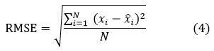
where, RMSE is Root- Mean Square Error, N is the number of data points, i is the ith variable, xi is the actual rainfall and xi^ is the forecast rainfall.
Results and Discussion
In this paper, ARIMA and other statistical techniques have been used to forecast and determine the optimal model in rainfall prediction over Kolkata on the basis of 120 years of annual rainfall. Before applying the ARIMA model for prediction, the basic assumptions were tested and then the model has been compared to various regression techniques and discussed.
Augmented Dickey Fuller Test (ADF Test)
The ADF test is a statistically significant test, that there is a hypothesis testing involved with a null hypothesis and alternative hypothesis and ‘p’ value are presented as a result of the test. In this study to check whether the annual rainfall data of Kolkata is stationary or not the ‘adfuller(d.dropna)’ function have been applied in python. As per the test the calculated ‘p’ value below 0.05 indicates rejection of the null hypothesis and acceptance of the alternative hypothesis. When the p-value is greater than the predetermined significance level (0.05), the null hypothesis cannot be rejected. The result of ADF test which has been performed in python is shown below (table 1) step by step:
Table 1: Augmented Dickey Fuller Test
| from statsmodels.tsa.stattool import adfuller |
| print(“p-value:”, adfuller (d.dropna()) |
| p-value: 0.00091 |
The table displays the code and tools utilized to obtain the p-value. Here, the calculated ‘p’ value is 0.00091 (Table 1), which is less than the significance level 0.05. So, it is inferred that the data is stationary as it rejects the null hypothesis and accept the alternative hypothesis.
Serial Correlation Analysis
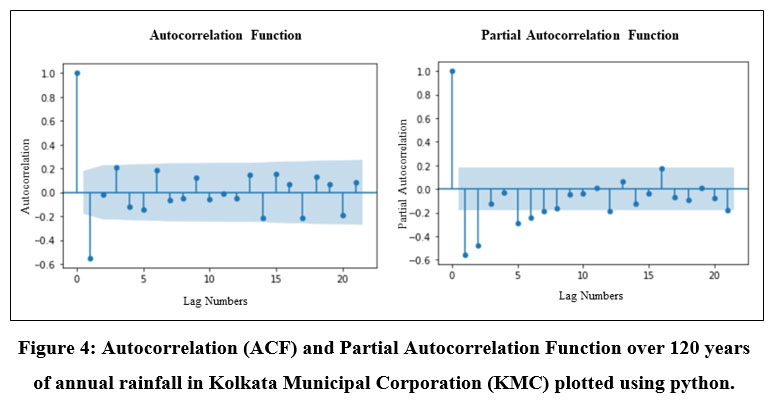
Serial correlation also known as autocorrelation is the correlation between two observations at different points in a time series data. When these auto correlations exist in data series it means that previous values have an impact on the current value. In the domain of time series analysis, it is prerequisite to study the autocorrelation and partial autocorrelation before modelling the series in order to get the better understanding about the datasets. These are mostly carried out to ensure that the presented data is a function of time and to provide evidence of that fact. Here, the annual rainfall over 120 years has a stationary pattern which means that there is no seasonal pattern and hence there is no need of differencing the data. The ACF and PACF which have been plotted to comprehend the auto correlation effect better as demonstrated below (Fig. 4):
 | Figure 4: Autocorrelation (ACF) and Partial Autocorrelation Function over 120 years of annual rainfall in Kolkata Municipal Corporation (KMC) plotted using python.
|
The above ACF and PACF have been calculated with import statsmodels and using function acf() and pacf() correspondingly and then plotted using plot_acf() and plot_pacf() function. The autocorrelation plot for 120 years of yearly rainfall in Kolkata Municipal Corporation is shown above (Fig. 4). The horizontal axis shows the lag numbers between the elements of the datasets and the vertical axis shows the value of the autocorrelated function which can range from -1 to 1. A vertical line corresponding to each lag is called a spike on the graph, which shows the value of autocorrelated function for that particular lag. The autocorrelation with lag zero is always one because it reflects the correlation between each term and itself. Statistical significance is assigned to each spike that rises above or falls below the significance zone. This indicates that the spike has a value that differs significantly from zero. When a spike is sufficiently away from zero it indicates presence of autocorrelation and when it is close to zero, it indicates absence of autocorrelation. So, from the above plot of autocorrelation of annual rainfall data over 120 years it is clears that all the spikes are closed to zero up to lag 21 except lag 1 which reflects that the data is not autocorrelated significantly. On the other hand, the PACF, which helps to determine the model terms shows the correlation between a sequence and itself over time. The partial autocorrelations for lags 1, 2, 3, 4 and 5 are statistically significant, and the other lags are very less significant as seen on the graph (Fig. 4). As a result, this PACF recommends fitting a fifth-order or sixth-order autoregressive model.
Rainfall Forecasting with ARIMA Model
In this study, the ARIMA model has been implemented in Python language and used to forecast rainfall. To achieve the best results, the basic parameters of this model p, d, and q has been determined, which are dependent on the nature of the time series data. To determine the best order for this model, import the auto_arima package from the pmdarima.arima library and use the stepwise_model.aic function, which finds the optimum order for the model automatically as shown in the following (table 2):
Table 2: Identification the optimum order for the best model of ARIMA using python
Identification the order of ARIMA model with performing stepwise search to minimize AIC | ||
Model | Order | AIC |
ARIMA | ARIMA (2,1,2) | 1763.918 |
ARIMA (0,1,0) | 1838.171 | |
ARIMA (1,1,0) | 1794.501 | |
ARIMA (0,1,0) | 1836.175 | |
ARIMA (1,1,1) | 1760.029 | |
ARIMA (0,1,2) | 1760.155 | |
ARIMA (1,1,2) | 1762.026 | |
ARIMA (0,1,1) | 1757.651 | |
ARIMA (1,1,2) | 1760.055 | |
The above results (Table 2) shows that the optimum order for the best model is 0, 1, 1 for the parameters of p, d and q respectively, which has the lowest AIC that is 1757.65 among the other orders. It has been then used as the order of the model with the function of stats ARIMA (df, order = (0,1,1) to get best results of the model. After determining the best model to forecast the rainfall it is required to validate the result. Therefore, the data has been divided into training data from 1901-2000 and test data from 2001-2020. After that, it produces the predicted annual rainfall for the above mentioned 20 years periods which is showed in the following table (Table 3) and then plotted the actual and forecasted annual rainfall which is shown in the following (Fig. 5):
Table 3: Forecasted annual rainfall from 2001 to 2020 as computed with ARIMA model using python
Years | Annual Rainfall (mm) | Years | Annual Rainfall (mm) | Years | Annual Rainfall (mm) | Years | Annual Rainfall (mm) |
2001 | 1806.57 | 2006 | 1762.87 | 2011 | 1594.92 | 2016 | 1503.62 |
2002 | 1751.94 | 2007 | 1739.23 | 2012 | 1316.87 | 2017 | 1450.18 |
2003 | 1800.19 | 2008 | 1708.44 | 2013 | 1515.97 | 2018 | 1509 |
2004 | 1804.12 | 2009 | 1676.96 | 2014 | 1427.7 | 2019 | 1470.8 |
2005 | 1778.07 | 2010 | 1661.78 | 2015 | 1415.65 | 2020 | 1482.85 |
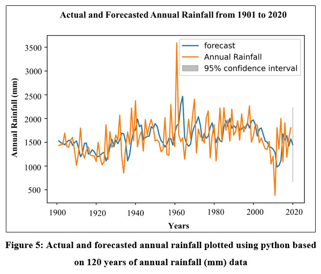 | Figure 5: Actual and forecasted annual rainfall plotted using python based on 120 years of annual rainfall (mm) data
|
The ARIMA model may be used for modeling and forecasting rainfall but to enhance the accuracy of new model and forecasts it must constantly update the previous data with new data and need to validate the results with observed data. This information about predicted rainfall can be used for urban planning purposes, such as flood management and rainwater conservation, in the research region.
Residual Diagnostics to check the Model
In this study, the standardized residuals, typical Q-Q plot and histogram plus estimated density has been plotted to assess the model residual diagnostics, which are shown in the following (Fig. 6):
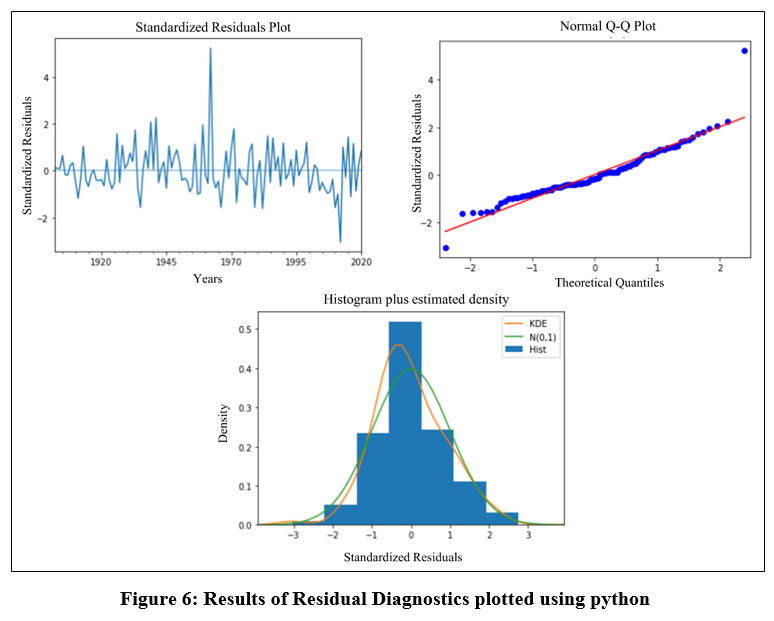 | Figure 6: Results of Residual Diagnostics plotted using python
|
The above normalized residual plot reflects that the residuals are independent since they are scattered in a random form, which is a prerequisite assumption for the ARIMA model to forecast the values. Here, the x-axis represents the forecasted value made by the model and the y-axis represents the accuracy of the prediction with standardized residuals. The larger the distance from the zero line reflects the worse prediction while the closer to zero reflects the better prediction. Except for two values for 1962 and 2012, the plot in this model indicates reasonable prediction because all of the values are between zero and plus or minus two.
The normal Q-Q plot indicates that all of the values with the exception of the first one or two and the last one is just around the 45-degree line, confirming the model's assumption that the data is normally distributed across the years 1901 to 2020.
The histogram plot along with estimated density reflects that the residuals are normally distributed which confirms the assumption of the model to predict the rainfall in this study. The normal density plot is shown on the green line, and the Kernel density estimation (KDE) plot is shown on the orange line, where the probability density function is represented on the y axis.
Linear and Polynomial Regression
In this study, simple linear regression and second-to-sixth-degree polynomial regressions have been employed (Fig. 7) to forecast the rainfall to determining the best model for effective forecasting. First, the 20 years of rainfall from 2001 to 2020 has been forecasted on the basis of 100 years of rainfall from 1901 to 2000 applying all of the above-mentioned techniques and then validated with actual rainfall from 2001 to 2020. So, in order to validate or to determine the best regression model the RMSE between actual rainfall and forecasted rainfall has been calculated with R square value for each of these regression models. The following are the graph of the last 20 years' projected annual rainfall from 2001 to 2020:
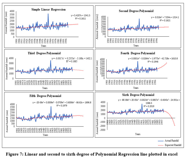 | Figure 7: Linear and second to sixth degree of Polynomial Regression line plotted in excel.
|
So, based on the above equations, the forecasted annual rainfall over the last 20 years from 2001 to 2020 has been determined for each regression model, which is as follows (Table 4):
Table 4: Forecasted annual rainfall from 2001 to 2020 as computed in Excel
Years
| Forecasted Annual Rainfall (mm) using various regression techniques | |||||
Linear trend | Second Degree Polynomial | Third Degree Polynomial | Fourth Degree Polynomial | Fifth Degree Polynomial | Sixth Degree Polynomial | |
2001 | 1346.92 | 1321.12 | 1399.17 | 1570.02 | 1633.71 | 1561.25 |
2002 | 1352.34 | 1328.10 | 1396.69 | 1533.03 | 1577.40 | 1535.67 |
2003 | 1357.76 | 1335.06 | 1394.67 | 1499.65 | 1527.47 | 1510.20 |
2004 | 1363.18 | 1341.98 | 1393.08 | 1469.64 | 1483.54 | 1485.22 |
2005 | 1368.60 | 1348.87 | 1391.93 | 1443.11 | 1445.22 | 1461.07 |
2006 | 1374.02 | 1355.73 | 1391.20 | 1419.62 | 1412.14 | 1438.03 |
2007 | 1379.44 | 1362.55 | 1390.87 | 1399.10 | 1383.97 | 1416.36 |
2008 | 1384.87 | 1369.35 | 1390.94 | 1381.40 | 1360.36 | 1396.26 |
2009 | 1390.29 | 1376.11 | 1391.41 | 1366.38 | 1341.00 | 1377.88 |
2010 | 1395.71 | 1382.84 | 1392.25 | 1353.87 | 1325.56 | 1361.36 |
2011 | 1401.13 | 1389.54 | 1393.46 | 1343.73 | 1313.74 | 1346.79 |
2012 | 1406.55 | 1396.20 | 1395.03 | 1335.82 | 1305.27 | 1334.21 |
2013 | 1411.97 | 1402.84 | 1396.95 | 1329.99 | 1299.86 | 1323.67 |
2014 | 1417.39 | 1409.44 | 1399.20 | 1326.11 | 1297.26 | 1315.14 |
2015 | 1422.81 | 1416.01 | 1401.79 | 1324.03 | 1297.20 | 1308.60 |
2016 | 1428.23 | 1422.55 | 1404.69 | 1323.62 | 1299.45 | 1303.98 |
2017 | 1433.65 | 1429.05 | 1407.89 | 1324.74 | 1303.77 | 1301.18 |
2018 | 1439.07 | 1435.53 | 1411.40 | 1327.27 | 1309.95 | 1300.11 |
2019 | 1444.49 | 1441.97 | 1415.19 | 1331.08 | 1317.77 | 1300.62 |
2020 | 1449.91 | 1448.38 | 1419.26 | 1336.04 | 1327.04 | 1302.56 |
Identification of Best Model
In this study, the coefficient of determination (R2) and Root Mean Square Error (RMSE) have been computed and considered to determine the optimum model for forecasting rainfall. The minimum RMSE is found with the fifth-degree polynomial equation, as shown in Table 5, among all the regression models. It is important to note that though the R2 (coefficient of determination) has increased with increasing degree of curvature from the straight line to sixth degree polynomial equation with higher r2 being 0.2019 at sixth degree polynomial equation but the lower RMSE is found at the fifth-degree polynomial equation. The value of r2 for the sixth-degree polynomial is maximum (Table 5) to express the degree of explained variance but the value of RMSE is not the least for the sixth-degree polynomial, which signifies that the sixth-degree polynomial regression is over fitting the 120 years of dataset. The RMSE for fifth degree polynomial is the least (Table 5) among all the polynomial equations, which entails that the fifth-degree curve is actually the best fit curve for forecasting the data, as it is neither an under fit nor an over-fit curve concerning its datasets. R-squared indicates how well a regression model explains the observed data or how well data fits the regression model. However, a big value of r-square does not always indicate a good regression model, which is proved in this study, as the quality of the statistical measure is dependent on a number of factors, including the nature of the variables used in the model, the units of measure used for the variables, and the data transformation used. The lowest RMSE has been found with fifth degree polynomial regression techniques that is 364.83 with compare to the other techniques or models. Although the ARIMA model have been used in this study and met all the requirements for forecasting rainfall but did not produce the best results. The r-squared value and RMSE has been shown in the following (Table 5).
Table 5: Order of ARIMA and Root mean square error with R square of various regression techniques calculated by the authors.
Trend Line/Model | Equation/order | R 2 | Root Mean Square Error (RMSE) |
ARIMA | P, d, q (0,1,1) | --- | 420.95 |
Linear trend Line | y = 5.4207x + 1341.5 | 0.1611 | 383.90 |
Second Degree Polynomial | y = -0.016x2 + 7.034x + 1314.1 | 0.1621 | 388.23 |
Third Degree Polynomial | y = -0.0017x3 + 0.2353x2 - 3.168x + 1402.1 | 0.1685 | 377.75 |
Fourth Degree Polynomial | y = 0.0001x4 - 0.0284x3 + 1.9775x2 - 42.728x + 1610.8 | 0.1946 | 367.16 |
Fifth Degree Polynomial | y = -2E-06x5 + 0.0006x4 - 0.0709x3 + 3.6006x2 - 66.62x + 1696.8 | 0.1979 | 364.83 |
Sixth Degree Polynomial | y = -8E-08x6 + 2E-05x5 - 0.0023x4 + 0.0857x3 - 0.4045x2 - 24.931x + 1586.5 | 0.2019 | 372 |
An analysis of the long-term rainfall trend and its variability is a prerequisite to determining the feasibility of rainwater harvesting. In this regard, identifying the best model to forecast rainfall is necessary. The result obtained through the analysis of this study may help the planners for sustainable management of the water resource of the study area. The forecasting must provide significant confidence to the administrators to build policies in KMC regarding rainwater harvesting to reduce urban floods and manage the city's water resources sustainably. Even the same study can be applied to other cities where the best forecasting model can be used for water resource management.
Conclusions
The primary objective of the present study was to assess and contrast the efficacy of the ARIMA model in relation to other regression methodologies, encompassing linear regression and polynomial regressions ranging from second to sixth degree, for rainfall forecasting in Kolkata. The research has been performed utilizing a dataset consisting of 120 years of long-term annual and monthly rainfall data, covering the time period from 1901 to 2020. In order to assess the efficacy of the models, the root mean square error (RMSE) was computed utilizing both the training and test datasets, encompassing the timeframe spanning from 2001 to 2020. The results suggest that out of all the regression methods examined for forecasting rainfall, the fifth-degree polynomial equation had the lowest root mean square error (RMSE), indicating its superior forecasting performance. In overall, this work offers significant insights into the relative effectiveness of various forecasting methods and highlights the potential of utilizing fifth-degree polynomial regression to enhance the precision of rainfall forecasting in Kolkata. It is crucial to note that while the ARIMA model met all of the assumptions in this study to forecast rainfall, the fifth-degree polynomial regression produced the best results when compared to ARIMA. On the other hand, while the r-squared value in the sixth-degree polynomial equation is higher than in the fifth-degree polynomial equation, the results showed that the RMSE in the fifth-degree polynomial regression is lower, indicating that this is the best model or technique for forecasting rainfall in this study. As a result, a consistently high r-squared value does not imply that this is the optimal prediction model. On the other hand, even if the ARIMA model fits all of its assumptions to predict rainfall, it does not always mean that it will always be the best model for forecasting rainfall. To recapitulate, rainfall forecasting is critical in Kolkata and since it is a city of urban flood during periods of heavy rainfall therefore it is essential to identify the appropriate model to forecast rainfall for effective water management.
Acknowledgement
We would like to thank Jadavpur University, Kolkata for providing all necessary facilities for this research work.
Conflict of Interest
There is no conflicts of interest to disclose.
Funding Sources
There is no financial support for publication of this paper.
References
- Huang NE, Shen Z, Long SR, et al. The empirical mode decomposition and the Hubert spectrum for nonlinear and non-stationary time series analysis. Proc R Soc A Math Phys Eng Sci. 1998;454(1971):903-995. doi:10.1098/rspa.1998.0193.
CrossRef - Serinaldi F, Kilsby CG. A modular class of multisite monthly rainfall generators for water resource management and impact studies. J Hydrol. 2012;464-465:528-540. doi:10.1016/j.jhydrol.2012.07.043
CrossRef - Zhang W, Villarini G, Vecchi GA, Smith JA. Urbanization exacerbated the rainfall and flooding caused by hurricane Harvey in Houston. Nature. 2018;563(7731):384-388. doi:10.1038/s41586-018-0676-z
CrossRef - Poornima S, Pushpalatha M. Prediction of rainfall using intensified LSTM based recurrent Neural Network with Weighted Linear Units. Atmosphere (Basel). 2019;10(11). doi:10.3390/atmos10110668
CrossRef - Ouyang Q, Lu W, Xin X, Zhang Y, Cheng W, Yu T. Monthly rainfall forecasting using EEMD-SVR based on phase-space reconstruction. Water Resour Manag. 2016;30(7):2311-2325. doi:10.1007/s11269-016-1288-8
CrossRef - Box, G. E. P., & Jenkins GM. Time series analysis: forecasting and control. San Francisco, CA: Holden-Day. [University Wisconsut Madison WI Univ ofLancaster, England]. 1976;(1970):1989.
- George E. P. Box et.al. C_2 Meteorological Applications - 2015 - Valipour - Long?term runoff study using SARIMA and ARIMA models in the United States.pdf. Published online 2016. doi:10.1111/jtsa.12194
CrossRef - Ayuba P, Journal MA-SW, 2018 undefined. Comparative analysis of the performance of artificial neural networks (ANNs) and autoregressive integrated moving average (ARIMA) models on rainfall forecasting. ScienceworldjournalOrg. 2018;13(1):100-105. http://www.scienceworldjournal.org/article/view/18415
- Bari SH, Rahman MT, Hussain MM, Ray S. Forecasting Monthly Precipitation in Sylhet City Using ARIMA Model. Civ Environ Res. 2015;7(1):69-78. http://www.iiste.org/Journals/ index.php/CER/article/view/19069
- Rahman MA, Yunsheng L, Sultana N. Analysis and prediction of rainfall trends over Bangladesh using Mann–Kendall, Spearman’s rho tests and ARIMA model. Meteorol Atmos Phys. 2017;129(4):409-424. doi:10.1007/s00703-016-0479-4
CrossRef - Wanders N, Bachas A, He XG, et al. Forecasting the Hydroclimatic Signature of the 2015/16 El Niño Event on the Western United States. J Hydrometeorol. 2017;18(1):177-186. doi:10.1175/JHM-D-16-0230.1
CrossRef - Kumar D, Singh A, Samui P, Jha RK. Forecasting monthly precipitation using sequential modelling. Hydrol Sci J. 2019;64(6):690-700. doi:10.1080/02626667.2019.1595624
CrossRef - Oswal N. Predicting Rainfall using Machine Learning Techniques. 2019;Book. doi:10.36227/techrxiv.14398304.v1
CrossRef - Nath P, Saha P, Middya AI, Roy S. Long-term time-series pollution forecast using statistical and deep learning methods. Neural Comput Appl. 2021;33(19):12551-12570. doi:10.1007/s00521-021-05901-2
CrossRef - Tharun VP, Prakash R, Devi SR. Prediction of Rainfall Using Data Mining Techniques. Proc Int Conf Inven Commun Comput Technol ICICCT 2018. 2018;(Icicct):1507-1512. doi:10.1109/ICICCT.2018.8473177
CrossRef - Srikanth P, Rajeswara Rao D, Vidyullatha P. Comparative analysis of ANFIS, ARIMA and polynomial curve fitting for weather forecasting. Indian J Sci Technol. 2016;9(15). doi:10.17485/ijst/2016/v9i15/89814
CrossRef - George J, Janaki L, Parameswaran Gomathy J. Statistical Downscaling Using Local Polynomial Regression for Rainfall Predictions – A Case Study. Water Resour Manag. 2016;30(1):183-193. doi:10.1007/s11269-015-1154-0
CrossRef - Joshi H, Tyagi D. Forecasting and Modeling Monthly Rainfall in Bengaluru, India: An Application of Time Series Models. Int J Sci Res Res Pap Math Stat Sci. 2021;(1):39-46. www.isroset.org
- Sinha S, Gupta O, Singh V, et al. A Comparative Analysis of Machine Learning Models for Solar Flare Forecasting: Identifying High Performing Active Region Flare Indicators. Published online 2021:1-15.
CrossRef - Litta AJ, Mary Idicula S, Mohanty UC. Artificial Neural Network Model in Prediction of Meteorological Parameters during Premonsoon Thunderstorms. Int J Atmos Sci. 2013;2013:1-14. doi:10.1155/2013/525383
CrossRef - Bhattacharya S, Bhattacharyya HC. A comparative study of severe thunderstorm among statistical and ANN methodologies. Sci Rep. 2023;13(1):1-14. doi:10.1038/s41598-023-38736-z
CrossRef - Choubin B, Zehtabian G, Azareh A, Rafiei-Sardooi E, Sajedi-Hosseini F, Ki?i Ö. Precipitation forecasting using classification and regression trees (CART) model: a comparative study of different approaches. Environ Earth Sci. 2018;77(8):1-13. doi:10.1007/s12665-018-7498-z
CrossRef - Md J Alam, Majumder A. Statistical analysis of rainfall trend and its variability (1901–2020) in Kolkata, India. Bull Geogr Phys Geogr Ser. 2022;23(23):5-16. doi:10.12775/bgeo-2022-0006
CrossRef - Anderson RL. Distribution of the Serial Correlation Coefficient. Ann Math Stat. 1942;13(1):1-13. doi:10.1214/aoms/1177731638
CrossRef - Sharma S, Singh PK. Long term spatiotemporal variability in rainfall trends over the state of Jharkhand, India. Climate. 2017;5(1). doi:10.3390/cli5010018
CrossRef - Zhang PG. Time series forecasting using a hybrid ARIMA and neural network model. Neurocomputing. 2003;50:159-175. doi:10.1016/S0925-2312(01)00702-0
CrossRef - Box, George E. P.; Jenkins, Gwilym M.; Reinsel GC. Time Series Analysis: Forecasting & Control (3rd Edition). Third Edit. Englewood Cliffs, N.J.?: Prentice Hall,; 1994.
- Akaike H. A New Look at the Statistical Model Identification. IEEE Trans Automat Contr. 1974;19(6):716-723. doi:10.1109/TAC.1974.1100705
CrossRef


