Current World Environment

Introduction

The death toll goes beyond seven million due to air pollution annually, with significant economic costs and health burdens, particularly in global south countries. This underscores the urgent need for action to mitigate these risks and protect health, noting that early exposure can lead to lifelong health issues. Air pollution is a pressing issue in India also, with approximately 80% of Indian metropolitan areas failing short of fulfilling the expected air quality benchmarks. Alarmingly, around 56% of these cities exceed permissible limits by nearly 1.5 times, leading to significant mortality and morbidity. North Central Maharashtra region has appeared in the research literature on various ecological and environmental aspects. Kaushik discussed the significant global issue of air pollution caused by anthropogenic activities, leading to severe health problems and a reduction in public subjective well-being.¹ A study measuring the atmospheric concentrations of lead, cadmium, nickel, manganese, and zinc in Aurangabad using high-volume air samplers was reported in literature.² High levels of these metals were found at various locations of heavy traffic and Industrial areas. Owing to the significant air pollution challenges, with particulate matter levels frequently exceeding national standards, detailed studies on air quality and preventive measures were recommended.³ While the aforesaid research articles touch upon various aspects regarding air quality management in non-attainment cities, a review of existing literature reveals limited published studies specifically addressing the air quality status of the North Central Maharashtra region, indicating a gap in publicly accessible scientific data for this area.

This knowledge gap necessitated a data-driven approach to understand the current state of air pollution, identify predominant sources, and evaluate existing control measures. However, the urgency of addressing air pollution extends beyond the absence of recent studies. The North Central Region of Maharashtra faces escalating environmental and public health concerns due to air pollution. Unfortunately, comprehensive and updated data on these pollutants in this region remains scarce. This lack of information hinders the development of effective mitigation strategies. The advancements in air quality monitoring technologies and analytical techniques now allow for a more detailed and accurate assessment of these pollutants. By filling this knowledge gap, the present study aims to provide critical insights that can inform policymakers, aid in progressive mitigation strategies, and ultimately contribute to the improvement of air quality and public health. The present study will be academically valuable andhold significant practical implications for environmental management and regulatory frameworks.

Despite the availability of national-level air quality data, there is a notable lack of region-specific investigations focusing on the North Central Maharashtra region. This area is experiencing rapid urbanization and industrial activity, yet localized studies that assess spatial and temporal patterns of air pollution are limited. Therefore, this study was designed to address the practical research problem of assessing ambient air quality in this region using a combination of ground-based monitoring and geospatial analysis. The findings aim to support evidence-based environmental planning and local pollution mitigation efforts.

Materials and Methods

The administrative boundary of the analysis zone was clipped from the global administrative boundary database available at Global Administrative Areas Database Management.⁴ The coordinates of the administrative boundary were reprojected to the UTM Zone 43N / WGS84 system. The satellite datasets obtained for this research, intended for integration, analysis, and interpretation, were clipped to match the edge extent of the administrative boundary of the study area. Air quality monitoring instruments were used to measure particulate matter (PM₁₀ and PM_2.5) concentrations. Envirotech Dust Sampler APM460 DXNL (PM₁₀) is a high-volume air sampler specifically designed for measuring particulate matter (Dust Particles) with a wind-flow dynamic diameter of smaller than 10 micrometers (PM₁₀). This instrument is equipped with a gaseous sampling attachment, enabling the simultaneous collection of gaseous pollutants along with particulate matter. The APM460 DXNL was set up and operated according to the manufacturer’s guidelines to ensure accurate and reliable data collection. The device's performance and calibration were periodically verified to maintain data integrity. Envirotech APM411TE, a robust and efficient air quality monitoring device, is a commercialized version of the CSIR – NEERI, a government of India initiative. This sampler is tailored for environmental research and commercial applications, offering precise measurements of various air pollutants. This instrument was used in order to get a reliable means to cross-validate data obtained from other instruments and to enhance the comprehensiveness of our air quality assessment. To monitor fine particulate matter (PM_2.5), the Envirotech Dust Sampler APM550 MFC (PM_2.5) was utilized. This fine particulate sampler is designed to capture particles with a wind-flow dynamic diameter less than 2.5 micrometers. The APM550 MFC operates with a mass flow controller, ensuring consistent and accurate sampling rates. This instrument's high sensitivity and precision made it an ideal choice for detecting fine particulate pollution, which is crucial for assessing health impacts and environmental quality. The instruments were deployed at the Jawaharlal Nehru Engineering College (JNEC) laboratory. Calibration was performed before the start of the sampling using standard procedures to ensure measurement accuracy. The APM460 DXNL and APM550 MFC were calibrated for their respective particulate size ranges, while the APM411TE was calibrated for general air quality parameters. The sampling was conducted over a continuous period, with each session lasting 24 hours to capture diurnal variations in particulate matter concentrations. The data was recorded and stored for subsequent analysis. The collected samples were analyzed using gravimetric methods for PM₁₀ and PM_2.5, which involved weighing the filters were used both before and after sampling to determine the mass of particulate matter. The gaseous pollutants sampled with the APM460 DXNL were analyzed using appropriate chemical methods. Out of the nine air quality monitoring stations in this region, five are situated in residential neighbourhoods, three are located in industrial zones, and one is placed in a rural area.⁵ These air quality monitoring stations installed in the region were also used to collect the data. The data was collected twice a week at these locations.

To ensure accurate and reliable measurements in our study, calibration, quality assurance and control (QA/QC) for air quality monitoring instruments were conducted. Calibration of the Envirotech Dust Sampler APM460 DXNL (PM10) was carried out using NIST-traceable test dust with a known particulate concentration. The instrument was set to operate with a standard flow rate of 1.2 cubic meters per minute (m³/min), and calibration involved comparing the instrument’s readings against a reference gravimetric method. The expected concentration for PM10 was set at 100 µg/m³. Calibration checks were performed before the start of sampling and at regular intervals every 24 hours throughout the study. The allowable deviation was ±5% from the reference value, and calibration logs, including pre- and post-calibration measurements, calibration coefficients, and error margins, are provided in the supplementary materials. For the Envirotech Dust Sampler APM550 MFC (PM2.5), calibration utilized a mass flow controller to maintain a constant flow rate of 16 liters per minute (L/min) and a PM2.5 size-selective inlet. The calibration was done using a certified calibration aerosol with known particle sizes and concentrations, with the expected concentration set at 50 µg/m³ as per the ISO 13137:2013 (“Performance evaluation of air quality continuous monitoring systems”) and US EPA PS -11 (“Specification and Test Procedures for PM₁₀ High Volume Samplers”), with traceability to NIST SRM 2786 reference aerosol. Calibration was verified before sampling and checked every 48 hours. Any deviations in the values greater than ±3% from the reference values prompted recalibration. Calibration data, including pre- and post-calibration measurements and coefficients, are detailed in the supplementary materials. The Envirotech APM411TE, used for general air quality parameters, was calibrated with standard air quality reference gases, CO, NO₂, and SO_2, at concentrations of 10 ppm, 5 ppm, and 2 ppm, respectively. The calibration procedure involved zeroing the instrument with clean air followed by exposure to reference gases. The instrument’s response was adjusted to match the reference concentrations. Calibration was performed before the sampling period and rechecked every 72 hours, with an allowable deviation of ±4% from the reference readingsin line with US EPA 40 CFR Part 58 Appendix A. Calibration results and verification data are included in the supplementary materials.

Sampling was conducted continuously over a 24-hour periodat each measurement session to capture diurnal variations in particulate matter concentrations. Measurements were taken every hour to document both peak and off-peak levels of particulate matter. Each sampling session lasted for 24 hours, ensuring comprehensive data collection. The research work provides a clear description of this hourly sampling process and its role in capturing the diurnal cycle of air pollutants. A rigorous QA/QC framework for the study was established. Data collection occurred at nine stations: five in residential neighborhoods, three in industrial zones, and one in a rural area. Sampling took place twice weekly at each station, focusing on PM₁₀, PM_2.5, and gaseous pollutants (CO, NO₂, SO₂). Routine maintenance of instruments, including filter changes and cleaning every 48 hours, was performed to ensure their proper functioning. Issues detected during the operation were promptly addressed with recalibration or repairs as needed. Data were electronically recorded and stored in a secure database with backup copies. QA/QC procedures included regular performance checks and data quality assessments. The APM460 DXNL maintained a deviation of less than ±5% from reference standards, the APM550 MFC showed deviations consistently within ±3%, and the APM411TE had a deviation from reference gases maintained at ±4%. Any anomalies in the data were investigated, and corrective actions, such as re-sampling or recalibration, were taken as necessary.

The selection of monitoring instruments, calibration procedures, and data processing methods was guided by established regulatory standards and peer-reviewed literature. The particulate matter sampler (APM 460 DXNL) was calibrated using a certified reference aerosol following US EPA Performance Specification 11 and ISO 13137:2013. Gaseous pollutant analyzers were calibrated with NIST-traceable gas standards in line with US EPA Methods 6C (SO₂), 7E (NO₂), and 10 (CO). Conversion of satellite imagery to TOA radiance was essential for enabling radiometric consistency and was performed according to Chander et al. and USGS Landsat Data Processing Guidelines, facilitating reliable comparison across dates and scenes. Spatial interpolation of air quality data was done using Inverse Distance Weighting (IDW), a well-established geostatistical method suited for environmental studies with unevenly distributed monitoring stations. The choice of IDW was based on its ability to provide reasonable estimates with minimal computational assumptions, as recommended in recent air quality mapping literature⁶².

Radiometric correction involves converting the magnitude of a Digital Number (DN) to the amount of radiance or reflectance magnitude. This process can be performed at each step change of radiance standardization. The first level involves converting sensor DN values to at-sensor radiances using sensor calibration data. The second level transforms at-sensor radiances to ground level radiance⁶.

Conversion to TOA Radiance: Conversion to Top-of-Atmosphere (TOA) Radiance was performed to transform the raw digital numbers (DNs) obtained from satellite imagery into physically meaningful radiometric units (W/m²·sr·µm). This step is essential for ensuring consistency across scenes acquired under different illumination conditions and sensor settings. TOA radiance accounts for the sensor’s spectral response and solar geometry, which is critical for any subsequent atmospheric correction, quantitative analysis, or temporal comparison of surface features.

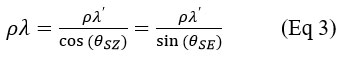
The metadata file includes radiance rescaling factors, which can be applied to transform OLI and TIRS band data were converted into top of atmosphere (TOA) reflectance^7-8

L_h= TOA spectral radiance (Watts/(m2 * srad * µm))

M_L = the valve of the band-specific multiplicative rescaling factor was obtained from the meta data

(RADIANCE_MULT_BAND_x, where x represents the specific band number)

AL = summative rescaling factor particular to the Band retrieved from the metadata

(RADIANCEADDBand), where x represents the specific band number.

Q_cal = Standardized and adjusted standard product pixel values (DN)

Conversion of TOA Reflectance

Band data can be converted to top-of-atmosphere (TOA) ground surface reflectance using reflectance rescaling factors available in the product metadata file (MTL file). The following formula illustrates the transformation of DN values into TOA reflectance for OLI data^9–11

ph'= TOA planetary reflectance, without correction for solar angle. Note that ph' does not contain a correction for the sun angle.

Mp =The band-specific multiplicative rescaling factor was extracted from the metadata.The band –specific multiplicative rescaling factor was extracted from the

(REFLECTANCE_MULT_BAND_x where x represents the specific band number)

Ap = summative rescaling factor particular to the Band retrieved from the metadata

(REFLECTANCE_ADD_BAND_x, x denotes the band number)

Qcal = Standardized and adjusted pixel values of the product (DN)

TOA reflectance, adjusted for the sun angleTOA reflectance, adjusted for the sun angle, is:^12,13

ph = TOA planetary reflectance

0SE = Local sun elevation angle measured in degree at the scence center is provided in the metadata SUN ELEVATION.

0SZ = Local solar zenith angle; 0SZ = 90° - 0SE

To improve reflectance estimates, utilize per-pixel solar angles instead of scene center angles. However, Landsat 8 does not presently offer per-pixel solar zenith angles.

Atmospheric Correction

It is important to note that Landsat 8 images includes band-specific rescaling factors ,which allow direct conversion from DN valve to Top-of-Atmosphere (TOA) reflectance. However, to accurately measure ground-level reflectance, the effects of the atmosphere, which can vary with wavelength, must be accounted for. As explained by Moran et al., the land surface reflectance (p) can be determined using these considerations.^14,15

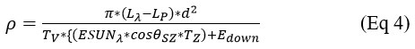
where:

LP = Radiance along the path

TV = Atmospheric opacity along the line of sight

TZ = Atmospheric opacity in the light source direction

Edown = downwelling diffuse irradiance

ESUNh= mean solar exo-atmospheric irradiances

d = The Earth_sun distance included in the Landsat 8 metadata,is used for reflectance calculation

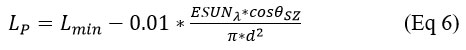
The Landsat 8 image's path radiance was calculated using the Dark Object Subtraction (DOS) technique.^16,17

Where,

L_min is the calibration constant (RADIANCE_MINIMUM_BAND_x, where x is the band number)

Several Dark Object Subtraction(DOS) techniques Such as DOS1, DOS2, DOS3, DOS4), are available,each based on  different assumptions regardingT_V, T_Z, and E_down.

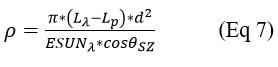
In this study, the method simplest technique is the DOS1, where the followingassumptions are made¹⁴: TV = 1; TZ = 1; Edown = 0. Therefore, the pathradiance is:

the resulting land surface reflectance is given by:

Aerosol Optical Thickness (AOT) and PM10 Correlation

The atmospheric reflectance was subsequently correlated with PM₁₀ concentration levels.The atmospheric reflectance was subsequently then correlated with PM₁₀ concentrations using regression analysis. PM₁₀ models were calculated based on this analysis. PM10 maps were generated using the proposed algorithm, selected for having the highest correlation coefficient (R = 0.888) and the lowest Root Mean Square Error (RMSE) values. The linear regression model, as presented by Nadzri O et al. (2010), is used for this purpose.

PM10 represent the concentration of particulate matter with a diameter of 10 micrometer or less, measured in microgram per cubic meter (µg/m³), while R h1, R h 2, and R h 3 are denote the Atmospheric reflectance/path radiance in the blue, green, and red spectral bands.

Sentinel-5P Sulfur Dioxide and Nitrogen Dioxide

The Sentinel-5P satellite, operated by the European Space Agency (ESA), is dedicated to monitoring atmospheric composition and air quality.⁶¹ The data obtained includes the Sentinel-5P OFFL SO2 and Sentinel-5P OFFL NO₂ products, which measure concentrations of sulfur dioxide (SO₂) and nitrogen dioxide (NO₂) in the atmosphere, respectively. SO₂ is a significant atmospheric pollutant primarily emitted by volcanic activity and the combustion of fossil fuels. NO2, another critical pollutant, originates largely from industrial activities and vehicle emissions. These products are processed in an offline mode, meaning the data is provided with a delay to ensure high accuracy and quality, making them suitable for detailed environmental and atmospheric studies.

The Sentinel-5P data for SO₂ and NO₂ was acquired through. Google Earth Engine (GEE), robust cloud-based platform designed for analysing environmental data analysis. The first step involved filtering the data based on specific time frames and geographic areas of interest, ensuring relevance to the study objectives. Cloud masking techniques were applied to exclude pixels affected by clouds, thus improving the reliability of the atmospheric data. The data was then reprojected to a common spatial reference system and re-sampled to a consistent resolution to facilitate uniform analysis.

For the analysis, concentration maps of SO₂ and NO₂ were created, providing a visual representation of pollutant levels across the study area. Temporal trends and seasonal variations were examined by calculating average concentrations over specific periods and identifying changes over time. Additionally, correlation and regression analyses were conducted to explore the relationships between pollutant concentrations and potential sources, such as industrial zones and traffic density. This analysis helped identify contributing factors to the observed pollution levels.

The study included validation and quality assessment steps, such as cross-verifying satellite data with available ground-based measurements to evaluate accuracy. An uncertainty analysis was also performed, considering potential errors due to factors like cloud cover, sensor calibration, and atmospheric conditions. The results were interpreted and reported using various visual tools, including maps and charts, to communicate the findings regarding the spatial distribution, temporal trends, and potential sources of SO₂ and NO₂. This comprehensive methodology leverages Sentinel-5P data and the capabilities of GEE to provide robust insights into air quality and atmospheric pollution.¹⁸

Spatial interpolation

Spatial estimation is a technique used to determine values at unmeasured locations by utilizing data from nearby or surrounding measured points. According to Tobler’s First Law of Geography, which suggests that locations closer in proximity are more likely to exhibit similar values than those farther apart, this method uses a neighborhood of sampled points to estimate values at unsampled sites.¹⁹ It is widely applied for predicting unknown data for geographical variables such as elevation, precipitation, chemical concentrations, and noise levels. The selection of an estimation method depends on factors like the available data, spatial and temporal resolution, desired output, and accuracy requirements.

To estimate pollutant levels at an unmeasured location, spatial interpolation techniques are employed. These techniques are broadly categorized into two types: deterministic and stochastic (non-deterministic).²⁰ Deterministic methods rely on explicitly defined spatial parameters, such as the level of similarity or smoothing applied. In contrast, stochastic methods incorporate random functions and account for spatial relationships between data points. Stochastic approaches analyse spatial autocorrelation among observed data points and consider the spatial arrangement of samples around the target location for prediction. Unlike deterministic methods, which do not provide error estimates for predicted values, stochastic methods offer both error evaluations and variance estimates for the predictions.

Thin plate spline interpolation

The Spline interpolation technique utilizes an interpolation method that estimates values using a mathematical function designed to reduce the overall surface curvature. This results in a continuous and even surface that exactly intersects the provided data points. The approach involves a weighted sum of thin plate splines, each centred on a data point, which generates an interpolation function that not only intersects the points but also minimizes the surface's bending energy. Although the fundamental requirement is that the spline must intersect all data points, regularization techniques can be introduced to relax this constraint, particularly in cases of noisy or sparse data.

The primary concept behind minimum curvature spline interpolation is based on two essential conditions: the surface must exactly intersect the data points, and the surface must exhibit minimal bending. More precisely, the method seeks to minimize the aggregate sum of the squared second derivatives of the surface across the entire domain. This ensures that the surface remains as gentle as possible while still adhering to the data points. Regularization allows for a trade-off between surface smoothness and fidelity to the data, which is particularly important when the data is irregular or incomplete. This method is widely used in areas such as spatial modellingand digital rendering, where generating surfaces that are both accurate and visually coherent is crucial.

Interpolation base on Inverse distance weighted

The Inverse Distance Weighted (IDW) interpolation method predicts the valve of cell at an undefined location by taking the mean of the values of data points in proximity.²¹ The closer a data point is to the centre of the cell being estimated, the greater its influence or weight in the averaging process. This method assumes that the closer a sample point is to the undefined location, the more reliable its value will be for estimating the value of that location.²² IDW is a widely used method in GIS and is often considered one of the simplest forms of interpolation. Various techniques utilize weighted moving averages of points within a defined area of influence. The IDW algorithm typically works by assigning weights to the surrounding data points based on their distance, with closer points receiving higher weights. IDW primarily the inverse of the distance raised to a certain power.²³ The exponent determines the extent to which nearby known points influence the interpolated value based on their distance. This exponent is always a positive real number with a default value of 2. By increasing the power, more emphasis is placed on nearby points, resulting in a more detailed (less smooth) surface. The higher the power value, the more the interpolation will mimic a “point-source” effect, where the interpolated value is dominated by very close samples. As the power value rises, the interpolated values will closely match the nearest sample point. Conversely, a lower power value allows more distant points to influence the result, producing a smoother surface. This characteristic makes IDW sensitive to the distribution of data, and if data points are too sparse or unevenly distributed, it may lead to inaccurate or misleading results.

If the observed values are v_i, where i=1,…,n at locations p_i:(x_i,y_i) where i = 1,…,n , then the value at an unknown point u is given as:

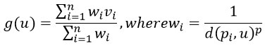
Usually, the most preferred value of p for IDW interpolation is 2, which has been considered and used in this study.

Kriging interpolation

Kriging is a spatial estimation technique that considers the distance along variation between known data points when predicting values in unknown areas. This method is grounded in the principles of geostatistics, which study the spatial dependency of data²³ models. In contrast to simpler approaches like Inverse Distance Weighted Interpolation, Linear Regression, or Gaussian decay models, Kriging relies on the spatial relationships between the sample points to make predictions across the area. It leverages the fact that nearby locations tend to have more similar values than those farther apart.²⁴ This approach emphasizes actual spatial arrangement of the data instead of relying on a predefined distribution model. One of the key advantages of Kriging is that it also provides estimates of the uncertainty associated with each predicted value, making it especially valuable in fields that require quantifiable confidence in the results, such as environmental science and resource management.²⁵

Recognized for its accuracy as an interpolator and "optimal linear predictor," Kriging calculates each predicted value by minimizing the error in the estimate. The objective is to reduce the prediction variance by considering both the known data and the spatial correlation structure.²⁶ For any given sampled location, the observed value will match the predicted value from Kriging, and all interpolated values are regarded as the best linear unbiased estimates. This optimality is achieved using weighted averages based on spatial autocorrelation, which reflects how spatial proximity influences the value of nearby points. Kriging operates in two main steps: first, a variogram is fitted to define the spatial covariance structure of the sample points, which captures the spatial variability of the data. The variogram helps to quantify the degree of correlation between points at different distances. Second, the weights derived from this structure are applied to predict values at unknown locations or areas within the spatial field, ensuring that the interpolation accounts for the inherent spatial patterns in the data.

Spatial pseudo-replication

Quasi-replication can be categorized into two types:

Terrestrial quasi-replication, which involves repeated measurements from the same subject or entity over time.

Space-related quasi-replication, which refers to multiple measurements taken within a similar spatial domain or region.

A significant challenge in pollution-related datasets is "space-related quasi-replication," commonly referred to as spatial autocorrelation, a critical concept in spatial statistics. Spatial autocorrelation describes the degree of correlation between values of a particular variable that arise due to their spatial proximity on a two-dimensional plane, which violates the assumption of spatial independence inherent in classical statistical analysis.²⁵ This phenomenon is crucial because it acknowledges that the value of a variable at one location can influence or be influenced by neighboring locations, thus violating the assumption of independence that is central to most statistical models. Essentially, data points that are geographically close to one another tend to be more highly correlated, whereas those farther apart exhibit lower correlation. This spatial dependence can introduce bias into the results of conventional statistical analyses.²⁶ Areas with closely positioned sampling points are termed hot spots, while regions with fewer measurement points are known as cold spots. Hot spots are densely sampled and often yield abundant data, while cold spots are sparsely sampled and more dispersed. Furthermore, observations from hot spots are likely to exhibit high similarity because they originate from nearly identical spatial locations, often reflecting similar environmental conditions or processes at those sites.

When neighboring data points exhibit similar values, this suggests positive spatial autocorrelation, indicating that similar environmental or spatial factors are influencing the area. On the other hand, significant differences between nearby observations suggest negative spatial autocorrelation, often indicating contrasting local conditions or processes. Detecting spatial autocorrelation is crucial because (a) it often suggests the presence of an underlying spatial pattern that merits further analysis to identify the causes of the observed spatial variability, such as natural environmental gradients or anthropogenic factors, and (b) it implies redundancy in the dataset, which has important implications for the selection of appropriate spatial analysis techniques and methodologies. Redundancy due to spatial autocorrelation can also affect the precision of estimations and the accuracy of predictive modelling, making it essential to account for spatial dependence in data analysis.

Variogram

A function that quantifies the relationship between the distance and direction separating two locations is used to measure spatial dependence. This concept is central to spatial statistics, where the degree of similarity between observations is often influenced by their relative positions. Spatial autocorrelation is typically modelledusing a fundamental tool known as the variogram. The variogram is defined as the variance of the difference between two observations at distinct spatial locations. This variance reflects how much the values of a variable at one location differ from those at another location as a function of the spatial separation. In general, the variogram increases as the distance between the locations increases, indicating that spatial dependence weakens as the distance grows. The variogram is characterized by three key parameters: nugget, sill, and range. The nugget represents the small-scale variability or measurement error, often attributed to very short-range spatial variations or observational inaccuracies. The sill indicates the maximum value the variogram reaches, representing the point at which the spatial correlation is essentially zero and beyond which increasing distance does not significantly affect the variance. The range defines the distance at which spatial correlation becomes negligible, and the variables become essentially independent. When the data is stationary (i.e., statistical properties do not change over space), the variogram and the covariance function are theoretically related. The covariance measures the joint variability of the variables at two locations, and, in a stationary setting, it is mathematically linked to the variogram through a specific relationship known as the semivariance, which is half the variance of the difference between values at two locations. Understanding these relationships is essential for accurate spatial modellingand interpolation.

The variogram describeshow rapidlyspatial autocorrelation decreases y(h) as the distance h. Here:

Nugget - small scale variation and measurement error.

Sill - asymptotic value of y(h), as h - 0o.

Range - the threshold distance beyond the data are no longer correlated.

The shape of a variogram must be asymptotic. If the variogram does not asymptote, then it indicates that the data is trended. For each combination of points in the collected dataset, the semi-variance (which measures half of the mean-squared difference between their values) is computed and graphed against the separation, referred to as the "lag," between them. The resulting graph of measured semi-variance values is called the "empirical" variogram, while the "theoretical" or "model" variogram represents the statistical model that best represents the observed distribution of the data.

Choice of variogram models

In spatial statistical analysis, estimating geographic data at locations lacking direct measurements depends on the parameters of a variogram model that aligns with the observed dataset.²⁷ Several variogram models can be considered, and the accuracy of the generated spatial map significantly hinges on selecting the most suitable model that accurately captures the spatial characteristics of the data. Although selecting a variogram model is often based on user preference, statistical tools are commonly  used to identify the most likely parameter Techniques such as quadratic error minimization, maximum likelihood estimation, and Bayesian inference are commonly utilized to identify the optimal model fit.^28,29 Three different variogram models, namely, the nugget effect, spherical and exponential models are prevalent. The nugget effect model is used for very small distances, the spherical effect model is used for a continuous but non-differentiable response variable, and the exponential model is used for a continuous and differentiable response variable. Furthermore, the documentation of the gstatpackage in R suggests the possibility of about 20 models, including Gaussian and Matern.³⁰ It was also suggested that despite the twenty models existing in R, not all of them are useful. However, in most cases, spherical, exponential and Maternmodels are useful.

Since the data collected in this study is only one-time, there is no significant assurance that the response variables PM10, SOX and NOX are Gaussian. Also, there is no sufficient information for the Matèrn model, which requires extra input parameters in R. Since emission effects are pretty much localized, the spherical model is considered the most suitable for this study.

Anisotropy

Since this is a study with pollutants, it is important to explore whether there is a directional effect in the intensity of pollution. If the sill varies with direction, the process exhibits zonal anisotropy, whereas if the range with direction it indicates geometric anisotropy. In this study, the stations where measurements have been taken, are scattered, and therefore zonal anisotropy is more of interest. Variograms in specific directions can be calculated with the help of R software.

North Central Maharashtra holds a prominent place in global tourismdue to its remarkable array of attractions, such as the rock-cut caves and temples in the mountain ravines of Ajanta and Ellora, the formidable Daulatabad Fort, and historical sites like the Bibi-ka-Maqbara. The region under consideration is situated at a latitude of 19°53'59" North and a longitude of 75°20' East on the banks of the Kham River, which is a tributary of the Godavari River. It is 512 meters above sea level, nestled among the extended hills of the Vindhya Range, with the Kham River flowing through it. The region under consideration covers a total land area of more than 139 km². The temperature of the Marathwada region is typically hot and dry. The average daily temperature ranges from 28°C to 38°C. An average annual rainfall of 734 mm occurs, while the relative humidity is extremely low for most of the year, ranging between 30% and 50%, but it peaks at 85% to 90% during the monsoon season. The forested area covers 557 km², accounting for only 7.6% of the total land area.North Central Maharashtra has a diverse economy with activities spanning various industries, tourism, education, and employment services.Rapid industrialization and urbanization have led to significant changes in the both physical development and population growth there has been a significant change in the physical growth and population. Current data reveals that the population of the region is around 1.2 million. There are numerous industrial and public units (small, medium, and large scale), residential areas, and public gardens, contributing to its dynamic urban landscape.

There is some arbitrary development of industrial sectors along the periphery of the south-western part of the region. Various automobiles, winery, chemical and pharmaceutical industries are functional in the industrial area, which can be primarily associated with air pollution. There are around 70 industry units, distilleries, breweries and electroplating industries. The Shendra MIDC, a new developing area, is 15 km away from Chhatrapati Sambhajinager and spans 600 hectares. The Railway Station MIDC, within AMC limits, covers 200 hectares and consists of many small, old, and sick industries. Chikalthana MIDC, also within AMC, covers 400 hectares and is an old industrial area. Waluj MIDC, located 12 km from the city, is a major industrial area covering 1500 hectares. A significant portion of carcinogens air pollutants is emitted dueto inadequate solvent recovery facilities and excessive solvent usage the improper facilities for solvent recovery in excess usage of solvent. A few preventive measures, such as increased efficiency of solvent recovery from 91% to 95%.and installation ofan evaporator for treatingspent wash, was initiated, thereby reducing the volume of spent wash requiring further treatment. The pharmaceutical industry, particularly is not counted under the ‘dirty’ class of industry as compared to many other industries.³¹ Still the expansion of this sector brings in newer challenges in controlling and preventing air pollution. The pharmaceutical industry releases Carbon monoxide, Nitrogen oxide, PM₁₀, Sulphur dioxide, volatile organic compounds, acid gases, fugitive emissions from pumps, solvent vapors, odiferous gases resulting from fermentation processes, and extraction solvent vapors.³² The Methodological Framework for Air Quality Assessment in North Central Maharashtra used in the present work is presented as figure 1.

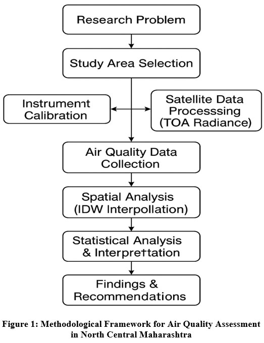Figure 1: Methodological Framework for Air Quality Assessment in North Central Maharashtra Click here to view Figure

Results and discussions

The high-resolution temporal variability and highlight short-term fluctuations in air quality in one week werestudied. The specific week chosen for detailed analysis, from 12 March 2023 to 23 March 2023, provided a snapshot of the spatial distribution of key pollutants and their concentrations, offering insights into the immediate impacts of local emission sources and meteorological conditions. This focused examination helped to identify acute pollution events and their sources, thereby complementing the broader, long-term trends observed over the two years.

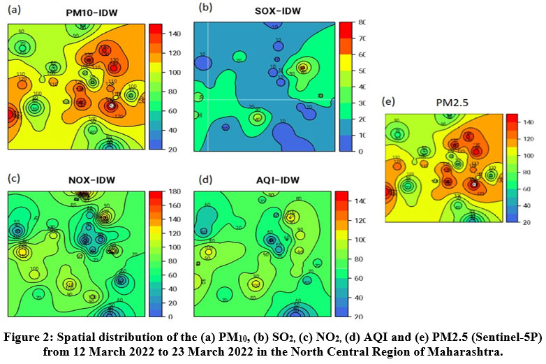Figure 2: Spatial distribution of the (a) PM10, (b) SO2, (c) NO2, (d) AQI and (e) PM2.5 (Sentinel-5P) from 12 March 2022 to 23 March 2022 in the North Central Region of Maharashtra. Click here to view Figure

Figure 2. illustrates the spatial distribution of various air quality parameters recorded by the Sentinel-5P satellite from 12 March 2023 to 23 March 2023 in the North Central Region of Maharashtra. The parameters included PM₁₀, SO₂, NO₂, Air quality index (AQI), and PM_2.5 concentrations. Each map used an Inverse Distance Weighting (IDW) interpolation method to represent the concentrations of these pollutants across the region. IDW interpolation method was applied to spatially represent pollutant concentrations, including SO₂, NO₂, PM₁₀, PM_2.5, and Aerosol Index (AI) across the region. IDW was chosen for its ability to estimate values at unsampled locations by giving higher weights to nearer data points, ensuring a more accurate representation of local variations in pollutant levels. This method allowed for the creation of continuous pollution maps, which are essential for visualizing spatial patterns and understanding the distribution of air quality across the study area. The spatial distribution of PM₁₀ showed several high-concentration hotspots, with values exceeding 140 µg/m³. These locations were primarily located in urban and industrial areas. This indicated significant emissions from vehicular traffic, industrial activities, and construction dust. In contrast, areas with lower PM₁₀ concentrations (20 to 60 µg/m³) were typically rural or less densely populated regions with lower emissions. The SO₂ concentration map revealed relatively lower overall concentrations compared to PM₁₀, with the highest levels (up to 8 µg/m³)in localized industrial zones, elevated concentration of sulfur dioxide (SO₂)emissions from the combustion of fossil fuel in power plants and factories. Most of the region exhibited lower SO₂ levels (0to 4 µg/m³), indicating lesser factories. The NO₂ concentration map showed a distribution pattern like that of PM₁₀, with high-concentration areas (up to180 µg/m³) in urban and industrial regions, indicative of emissions from vehicular exhaust and industrial processes. Lower NO₂ concentrations (20 to 60 µg/m³) were predominantly in rural areas with minimal traffic and industrial activities. The AQI map, integrating multiple pollutant concentrations, highlighted regions with poor air quality (AQI values exceeding 140), consistent with PM₁₀ and NO₂ hotspots. Areas with AQI values between 20 and 70 corresponded to regions with relatively better air quality, typically rural or less industrialized. The PM_2.5 distribution closely mirrored that of PM₁₀, with high concentrations (up to 140 µg/m³) in urban and industrial regions, posing significant health risks due to the fine particulate matter's ability to penetrate deeper into the respiratory system. Lower PM_2.5 concentrations (20 to 60 µg/m³) were generally found in rural areas with limited sources of fine particulate matter. The correlation between the PM₁₀ and PM_2.5 maps suggested that similar sources contributed to both size fractions. Elevated levels of NO₂ and SO₂ in specific areas indicated localized pollution sources, such as traffic congestion and industrial emissions.

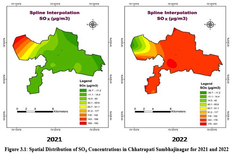Figure 3.1: Spatial Distribution of SO2 Concentrations in Chhatrapati Sambhajinagar for 2021 and 2022. Click here to view Figure

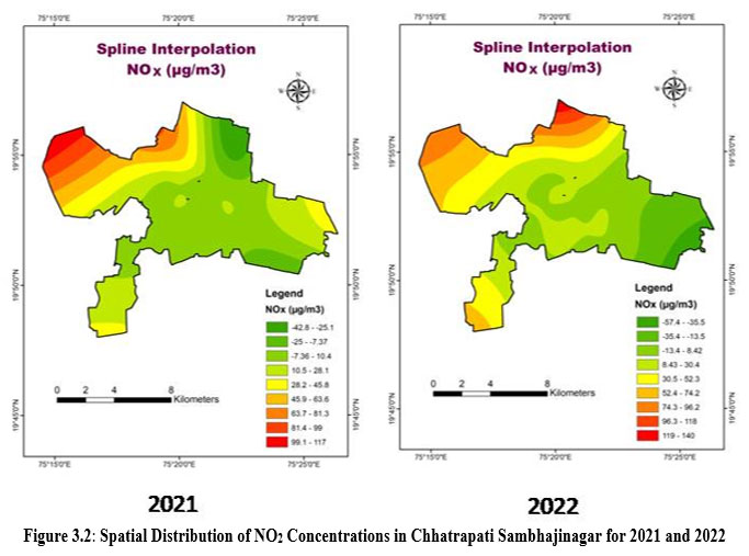Figure 3.2: Spatial Distribution of NO2 Concentrations in Chhatrapati Sambhajinagar for 2021 and 2022 Click here to view Figure

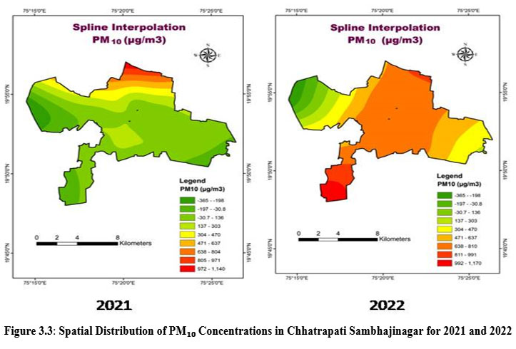Figure 3.3: Spatial Distribution of PM10 Concentrations in Chhatrapati Sambhajinagar for 2021 and 2022 Click here to view Figure

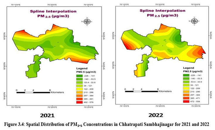Figure 3.4: Spatial Distribution of PM2.5 Concentrations in Chhatrapati Sambhajinagar for 2021 and 2022 Click here to view Figure

The analysis of spline interpolation maps Figures 3.1, 3.2,3.3 and 3.4) for SO₂, NO₂ and PM₁₀, over the Chhatrapati Sambhajinagar region from 2021 to 2022 revealed an alarming trend of increasing air pollution levels. The data highlighted the impact of industrial activities, vehicular emissions, and construction on air quality. The spline interpolation imagesunderscored an alarming increase in air pollutant concentrations across the Chhatrapati Sambhajinagar region from 2021 to 2022. Each pollutant—SO₂, NO₂ and PM₁₀,—showed a significant rise in concentration levels and an expansion in the spatial extent of high-concentration areas. The increase in SO₂ levels, especially in the central and western regions, was likely due to intensified industrial activities, vehicular emissions, and possible changes in fuel types or combustion efficiency. The central region's rise in SO₂ levels may have indicated either the diffusion of pollutants or the introduction of new pollution sources, exacerbated by westerly winds carrying emissions from industrial areas.The broader spatial increase in SO₂ concentrations suggested heightened vehicular emissions and industrial activities. The spread towards northern and eastern parts indicated either a shift in pollution sources or an increase in local activities contributing to NO₂ emissions, with prevailing wind directions playing a significant role in dispersing these pollutants. The substantial rise in PM₁₀ levels, especially in central and western parts, pointed to increased construction activities, vehicular emissions, and potentially agricultural practices contributing to particulate matter pollution. Wind patterns significantly contributed to the wide distribution of PM₁₀ across the region.

The spline interpolation images revealed a significant spatial distribution of NO₂ concentrations for the years 2021 and 2022. As seen in  figure 3.1the largest area coverage, characterized by NO₂ range of concentration 128.35–174.60 µg/m³, was found to span approximately 635.69 km², accounting for 42.86% of the total study area. This moderate class concentration predominantly affected most of the region. The high-value NO₂ class, with concentrations ranging from >249.10 to 362.57 µg/m³, was observed to cover about 93.48 km² or 6.30% of the area. The moderately low range of concentration 89.82–128.35 µg/m³ was found to cover 391.84 km² (26.42% of the area). The moderately high concentration range of 174.60–249.10 µg/m³ encompassed 140.61 km² (9.48% of the area). The low concentration range of 23.51–89.81 µg/m³, covering 14.93% of the study area, was found in certain other regions. These areas were largely impacted by mixed land-use patterns,Encompassing both commercial and residential  areas as wellas regions eith , heavy traffic flow.

The spatial analysis of PM₁₀ concentrations indicated that the highest concentration range (203.99–422.42 µg/m³) was localized in certain districts, covering a minimal area of about 22.90 km² (1.54%) (Figure 6.2). In contrast, the lowest range of concentration (22.82–43.05 µg/m³) was found to cover 30.05% of the area. The moderately high range of concentration (116.07–203.99 µg/m³) was observed in most of the regions, accounting for about 5.22% of the total area. The classes of PM₁₀, moderately low and moderate concentration classes with ranges of 43.05–69.87 µg/m³ and 69.87–116.07 µg/m³ respectively, were found to collectively cover 63.18% of the area, with 648.62 km² (43.74%) under the moderately low class and 288.39 km² (19.44%) under the moderate class. Notably, approximately 25% of the area had PM₁₀ levels exceeding the NAAQS permissible limit of 100 µg/m³ for a 24-hour average. The spatial distribution of PM_2.5 indicated that the moderately low concentration range (156.75–198.71 µg/m³) covered 627.34 km² or 42.30% of the total area. This range predominantly affected most of the region (Image 6.3). The moderate concentration range (198.71–253.43 µg/m³) spanned 133.33 km². The low concentration range (52.78–156.75 µg/m³) was found over 549.17 km² (37.03%). The moderately high concentration class (7.48% of the total area) was observed in certain areas, while the high concentration class, covering about 4.19% of the area, was found in others. Notably, except for marginal areas (approximately 3% of the total area), PM_2.5 concentrations surpassed the limit for the annual and 24-hour average ambient air quality standards.

Sulfur dioxide (SO₂)

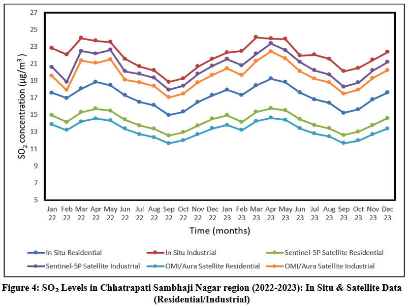Figure 4: SO2 Levels in Chhatrapati Sambhaji Nagar region (2022-2023): In Situ & Satellite Data (Residential/Industrial) Click here to view Figure

Sulfur dioxide (SO₂) is a significant air pollutant known for its harmful impacts on both the environment and human health.³³ Emitted primarily from industrial processes and the burning of fossil fuels, SO₂ contributes to acid rain, respiratory problems, and various other ecological and health issues.³⁴ SO₂ can adversely affect sensitive groups, such as the young, elderly, and those with asthma, even at low levels, making real-time monitoring essential. The burning of coal produces large amounts of SO₂ pollutants. The brick-making industry is largely associated with SO₂ emission. This emission mainly results from the combustion of sulphur-containing fuels such as coal or other fossil fuels, commonly used in the brick kilns.³⁵ Figure no.4 represents the SO₂ Levels in the Chhatrapati Sambhaji Nagar region for two consecutive years, 2022 and 2023. The data is presented for in situ and satellite data in residential as well as industrial areas. The analysis of the SO₂ concentration graph reveals significant seasonal variation. Across both years of data, SO₂ levels were observed to be higher during the colder months (November to February) and lower in the warmer months (May to August). This seasonal trend was consistent in residential as well as industrial areas. The elevated SO₂ concentrations during the colder months can be attributed to increased heating activities, which result in higher emissions of SO₂. Conversely, during the warmer months, the reduced need for heating, potentially lower industrial activity, and enhanced atmospheric dispersion likely contribute to the lower SO₂ levels. The proximity to industrial zones and the level of urbanization significantly influence the observed SO₂ levels. The data consistently showed higher SO₂ concentrations in industrial areas compared to residential areas. For instance, in January 2022, in situ measurements recorded SO₂ concentrations of 22.82 µg/m³ in industrial areas, whereas residential areas recorded 17.58 µg/m³. This trend was mirrored in satellite data, with Sentinel-5P and OMI/Aura showing similar differences between industrial and residential areas.

A persistent difference in SO₂ concentrations between residential and industrial areas was also vivid in the graph. This disparity is also evident in satellite data, underscoring the significant contribution of industrial activities to SO₂ emissions and the resultant air quality degradation in these regions.Both in situ measurements and satellite data provide valuable insights into SO₂ concentrations, each with distinct characteristics and utilities. In situ data offered high spatial and temporal resolution at specific locations, allowing for direct and highly accurate measurements. However, this approach has limited spatial coverage and requires extensive ground-based infrastructure and maintenance. In contrast, satellite data, including that from Sentinel-5P and OMI/Aura, offered wide spatial coverage, making it useful for monitoring large areas and remote or inaccessible regions. While satellite data has a lower spatial resolution compared to in situ measurements and can be affected by cloud cover and atmospheric conditions, it remains crucial for broad-scale air quality monitoring.The Sentinel-5P and OMI/Aura satellites both contribute significantly to SO₂ monitoring, though they have different strengths and limitations. Sentinel-5P, with its higher spatial resolution, provided more detailed observations, which were valuable for analysing localized pollution sources. Its more recent technology also suggests potential improvements in sensitivity and accuracy. However, it might have a slightly lower temporal resolution compared to OMI/Aura.OMI/Aura possesses potentially higher temporal resolution,allowingfor more frequent observations. Its lower spatial resolution compared to Sentinel-5P was indicative of the fact that it provided less detailed spatial information.³⁶

A comparison of SO₂ levels in January 2022 and January 2023 revealed relative stability in residential areas, with a slight increase from 17.58 µg/m³ to 17.94 µg/m³ in situ. In industrial areas, there was a slight decrease from 22.82 µg/m³ to 22.3 µg/m³ in situ. Satellite data from Sentinel-5P and OMI/Aura also reflected these trends, with minor variations. Monthly trends indicated that SO₂ levels peak during the colder months and reach their lowest levels during the warmer months. Industrial areas maintain higher SO₂ concentrations compared to residential areas throughout the year. Satellite data generally showed slightly lower SO₂ concentrations than in situ measurements, likely due to the spatial averaging inherent in satellite observations. However, both Sentinel-5P and OMI/Aura provided trends consistent with in situ measurements, affirming their reliability for broader spatial analysis. The SO₂ concentration data highlighted significant seasonal variations, geographical differences, and discrepancies between residential and industrial areas. In situ and satellite data were both crucial for comprehensive air quality monitoring. Sentinel-5P's higher spatial resolution provided finer detail, while OMI/Aura's extended data record offers valuable long-term insights. Combining these results in a more robust understanding of SO₂ pollution patterns was essential for developing effective mitigation strategies.

Temperature, humidity, wind speed, wind direction, rain, andevaporation are critical meteorological parameters. In the research study, the weather data were obtained from the India Meteorological Department website.³⁷ It releases daily weather variables for all the districts of all states of India. Conducting both Pearson and Spearman's correlation analyses was essential to understand the relationships between SO₂ concentration in the air and various meteorological parameters. In a residential area, the Pearson analysis revealed a weak, non-significant positive correlation with wind speed (r= .27, P = .20) and strong, significant correlations with average relative humidity (r= -.83, P = .00), average precipitation (r= -.62, P = .00), and average temperature (r= .69, P = .00). Spearman's analysis supported these findings, showing a non-significant positive correlation with wind speed (r_s = 0.18, P = 0.40889) and significant correlations with average relative humidity (r_s = -0.89, P < 0.001), average precipitation (r_s = -0.62, P = 0.00), and average temperature (r_s = 0.51, P = 0.01). In an industrial area, the Pearson analysis showed a weak, non-significant positive correlation with wind speed (r= .22, P = 0.30) and strong, significant correlations with average relative humidity (r= -.83, P < .00), average precipitation (r= -.60, P = .00), and average temperature (r= .65, P = .00). These results highlighted the critical impact of weather patterns on SO₂ pollution, with significant negative associations observed with humidity and precipitation, and positive associations with temperature, in both residential and industrial areas.

Nitrogen dioxide (NO₂)

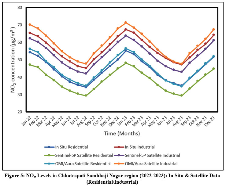Figure 5: NO2 Levels in Chhatrapati Sambhaji Nagar region (2022-2023): In Situ & Satellite Data (Residential/Industrial) Click here to view Figure

Nitrogen dioxide (NO₂) is a harmful air pollutant that impacts both the environment and human health.^38,39 It contributes to ozone and particulate matter formation and can directly affect the respiratory system upon inhalation. This makes monitoring NO₂ concentrations very crucial to understand its impact and develop control strategies. Figure 5 presented a comparison of NO₂ pollution levels in Chhatrapati Sambhaji Nagar across two years (2022 and 2023). The data is categorized by measurement approach (in situ and satellite) and location type (residential and industrial areas). This allows for a comprehensive examination of NO₂ variations over time and space. It is revealed by the NO₂ concentration data that a clear connection exists between seasons and air quality. NO₂ concentrations display pronounced seasonal and monthly variations. The patterns of NO₂ levels are influenced by the time of year.⁴⁰ Winter months (December to February) are shown to be the period with the highest NO₂ levels. Residential areas reach peaks as high as 55.23 µg/m³ in January 2023, while industrial zones are shown to soar even higher, reaching 67.32 µg/m³ during the same month. A combination of factors likely contributes to these elevated winter concentrations. Increased heating demands during colder months could lead to a rise in emissions from fuel combustion for residential heating. Additionally, winter often brings about temperature inversions, which are then observed to trap pollutants near the ground and hinder their dispersion into the atmosphere. This stagnant air further exacerbates the problem. Conversely, summer months (June to August) witness a dramatic drop in NO₂ levels, with residential areas dipping as low as 34.23 µg/m³ in August 2022 and industrial areas reaching 45.12 µg/m³. The rainy season, coinciding with the summer months, likely plays a significant role in this decline through the washout effect of rainfall, effectively cleansing the air of pollutants. Examination of NO₂ concentrations reveals a striking geographical disparity. Population density contributes to NO₂ emissions, still, industrialization was a greater cause due to the high-temperature combustion processes involved in many industrial activities.⁴¹ Industrial zones are consistently shown to demonstrate significantly higher levels compared to residential areas.⁴² This pattern is corroborated by both in situ and satellite measurements. For instance, in January 2022, in situ measurements revealed 65.34 µg/m³ in industrial areas, compared to 54.23 µg/m³ in residential areas. Similar discrepancies are observed in satellite data, with Sentinel-5P showing 62.15 µg/m³ for industrial zones and 47.12 µg/m³ for residential areas. This disparity can most likely be attributed to the concentrated presence of industrial activities, heavy traffic, and other localized sources of NO₂ emissions that are more prevalent in industrial zones.⁴³

The need to use multiple satellite datasets to improve the accuracy and study the human health effects of NO₂ exposures was reported by Zhongyu Huang et al.⁴⁴ It was also revealed that both in situ and satellite data play crucial roles in monitoring NO₂ concentrations, with their strengths and limitations.⁴⁵ In situ measurements offer the advantage of high spatial and temporal resolution for specific locations. This allows for highly accurate and direct measurements, providing valuable insights into localized variations in NO₂ levels. However, a significant drawback of in situ measurements is their limited spatial coverage.⁴⁶ The uneven distribution of ground-based monitoring stations could introduce errors in representing overall air quality.⁴⁴ Extensive ground-based infrastructure is required for widespread data collection, making it challenging to monitor large or remote areas. Satellite data, on the other hand, was shown to offer a wider spatial coverage, making it a valuable tool for monitoring NO₂ concentrations across vast regions, including remote and inaccessible areas. This is particularly beneficial for areas where establishing in situ monitoring stations might be impractical. However, satellite data presented NO₂ concentrations that are slightly lower than in situ measurements. This discrepancy is likely due to the inherent spatial averaging that occurs during satellite observations. While a satellite can measure NO₂ levels over a large area, it cannot capture the fine-grained variations that might exist within that area. Sentinel-5P data, for example, while offering high spatial resolution compared to other satellite sources, might still underestimate NO₂ concentrations compared to highly localisedin situ measurements. A detailed analysis of the data reveals significant year-over-year and seasonal changes in NO₂ concentrations. This suggested the fact that there was a potential rise in NO₂ emissions over time, highlighting the need for stricter regulations or cleaner technologies. Furthermore, the overall percentage change across the seasons indicated substantial variations. Winter months experience increasedbyup to 20% compared to summer months. This reinforces the earlier observation that seasonal factors significantly impact NO₂ levels. Additionally, the data consistently shows that industrial areas maintain higher NO₂ concentrations throughout the year compared to residential areas, highlighting the persistent influence of localized emission sources in these zones. Interestingly, satellite data, despite showing generally lower values than in situ measurements, aligns well with the observed trends. This convergence strengthens the case for using satellite data as a reliable tool for monitoring broad-scale air quality patterns. Satellite data inherently has drawbacks compared to in situ data collections, such as significant data gaps caused by cloud cover or other retrieval limitations.⁴⁷

The relationships between NO₂ concentration in the air and various meteorological parameters in both residential and industrial areas wereanalysed with the help of Pearson and Spearman's Rho correlation analyses. In residential areas, the Pearson analysis revealed strong, significant negative correlations with wind speed (r= -.74, P = .00), average relative humidity (r= -.69, P = 0.00), and average precipitation (r= -.86, P < .00), but a weak, non-significant negative correlation with average temperature (r= -.15, P = .47). These findings were supported by Spearman's Rho analysis, which showed similar significant negative correlations for wind speed (rs = -.75, P = .00), average relative humidity (rs = -.65, P = .00), and average precipitation (rs = -.92, P < 0.00), with a non-significant negative correlation for average temperature (rs = -.18, P = .41). In industrial areas, the Pearson analysis also revealed strong, significant negative correlations with wind speed (r= -.75, P =.00), average relative humidity (r= -.68, P = .00), and average precipitation (r= -.85, P < .00001), and a poor, non-significant negative correlation with average temperature (r= -.17, P = .44). Spearman's Rho analysis confirmed these findings, showing significant negative correlations for wind speed (rs = -.75, P = .00), average relative humidity (rs = -0.65, P = 0.00), and average precipitation (rs = -.92, P < 0.00), with a non-significant negative correlation for average temperature (rs = -.18, P = .39). Negative associations of NO₂ concentration were observed with wind speed, relative humidity, and precipitation, and non-significant associations with temperature, in both residential and industrial areas.

PM₁₀

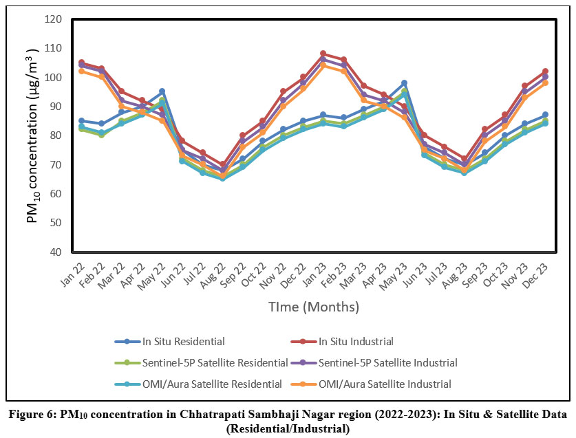Figure 6: PM10 concentration in Chhatrapati Sambhaji Nagar region (2022-2023): In Situ & Satellite Data (Residential/Industrial) Click here to view Figure

PM₁₀ air pollution has a detrimental impact on human health, contributing to a multitude of diseases. Studies have demonstrated that increased levels of PM_2.5 and PM₁₀ can lead to the onset of various diseases, including lung cancer,⁴⁸ asthma,⁴⁹ pneumonia,⁵⁰ hypertension,⁵¹ Alzheimer’s,⁵² and Parkinson’s disease.⁵³ As evident from Figure 6, the PM₁₀ concentration data revealed significant seasonal variations, geographical differences, and discrepancies between residential and industrial areas. Both in situ and satellite data were essential for comprehensive air quality monitoring, each offering unique advantages. The effectiveness comparison of the satellite and ground-based measurements forsensing air pollutants and their health hazards was recently carried out by Mushtaq et al.⁵⁴ Sentinel-5P's higher spatial resolution provided finer detail, while OMI/Aura's extended data record offered valuable long-term insights. Combining these data sources resulted in a more robust understanding of PM₁₀ pollution patterns, which was critical for developing effective mitigation strategies. In situ residential measurements showed PM₁₀ concentrations peaking at 87 µg/m³ in January 2023, while in situ industrial measurements reached as high as 108 µg/m³ during the same month. This seasonal trend was also reflected in satellite data, with Sentinel-5P recording 85 µg/m³ and 106 µg/m³ for residential and industrial areas, respectively, in January 2023 and OMI/Aura showing similar values. The winter peaks could be attributed to increased heating activities, stagnant air conditions due to temperature inversions, and possibly increased emissions from both residential heating and industrial processes. Conversely, the lower summer and rainy season levels, with residential in situ measurements dropping to 68 µg/m³ in August 2022, were likely explained by better atmospheric dispersion and the washout effect of rain.

Geographical factors significantly influenced PM₁₀ concentrations, with notable differences observed between residential and industrial areas. Industrial areas consistently showed higher PM₁₀ levels compared to residential areas. For instance, in January 2022, in situ measurements recorded 105 µg/m³ in industrial areas compared to 85 µg/m³ in residential areas. This pattern was mirrored in satellite data, with Sentinel-5P recording 104 µg/m³ for industrial areas and 82 µg/m³ for residential areas during the same month. These differences were likely due to higher emissions from industrial activities, including manufacturing processes, heavy traffic, and other localized sources of PM₁₀ in industrial zones. The data highlighted a significant difference in PM₁₀ concentrations between residential and industrial areas. Industrial areas consistently showed higher PM10 levels across all months and data sources. This difference was particularly pronounced during the winter months. For example, in January 2023, industrial areas recorded 108 µg/m³ in situ compared to 87 µg/m³ in residential areas. Satellite data from Sentinel-5P and OMI/Aura also showed higher PM₁₀ levels in industrial areas, underscoring the impact of industrial emissions. Residential areas, while having lower PM₁₀ concentrations, still exhibited significant levels likely due to traffic emissions and household activities such as cooking and heating.

Both in situ and satellite data were crucial for monitoring PM₁₀ concentrations, each offering unique advantages and limitations. In situ measurements provided high spatial and temporal resolution at specific locations, allowing for direct and highly accurate assessments. However, these measurements were limited in spatial coverage and required extensive ground-based infrastructure. Satellite data, including that from Sentinel-5P and OMI/Aura, offered wide spatial coverage, making them invaluable for monitoring large areas, including remote and inaccessible regions. However, satellite data typically showed slightly lower PM₁₀ concentrations compared to in situ measurements due to the spatial averaging inherent in satellite observations. For instance, in January 2023, in situ residential data recorded 87 µg/m³, while Sentinel-5P and OMI/Aura recorded 85 µg/m³ and 84 µg/m³, respectively. The Sentinel-5P and OMI/Aura satellites both significantly contributed to PM₁₀ monitoring, each with distinct benefits. Sentinel-5P, with its higher spatial resolution, provided more detailed observations that were crucial for identifying localized pollution sources. However, it may have had a slightly lower temporal resolution compared to OMI/Aura. OMI/Aura, with its longer operational history, offered a more extended time series of data, which was invaluable for long-term trend analysis. It also potentially offered higher temporal resolution, allowing for more frequent observations. Despite their differences, satellite data showed consistent trends within situ data, which further validated their utility in air quality monitoring.

A significant seasonal and year-over-year change in PM₁₀ concentrationswas observed. From January 2022 to January 2023, there was an approximate increase of 2.4% in residential areas (from 85 µg/m³ to 87 µg/m³) and 2.9% in industrial areas (from 105 µg/m³ to 108 µg/m³). The overall percentage change across seasons indicated substantial variations, with winter months experiencing increases of up to 25% compared to summer months. This seasonal fluctuation highlightedthe importance of considering temporal changes when assessing air quality. Consistently higher PM₁₀ concentration was observed in industrial area as compared to residential area throughout the year. Satellite data showed slightly lower PM10 concentrations than in situ measurements but aligned well with the observed trends, confirming the reliability of satellite observations for broad-scale air quality monitoring. The observed seasonal dependency and trend seemto be a global phenomenon influnced by seasonal variations in emissions and physical factors such as boundary layer height, 10-meter wind gusts, surface solar radiation, total cloud cover, wind divergence, sea level pressure, and precipitation.^55–57 A higher boundary layer and stronger surface wind gusts facilitate the rapid dispersion of PM10. Cloud cover and precipitation suggest that PM₁₀ dispersion is less efficient during the April to September period. PM₁₀ concentrations were lower during this period compared to other seasons. One possible reason for the lower PM₁₀ concentrations is the frequent convective activities during this season.⁵⁸ Early rainy season in this region causes frequent precipitation which helps wash out PM₁₀, reducing its concentration. In winter, atmospheric conditions favour PM₁₀ dispersion; wind gusts are strongest, wind divergence is highest, and sea level pressure is elevated. These conditions support the dispersion of locally produced PM₁₀. Despite these favourable conditions for horizontal dispersion, PM₁₀ concentrations were higher than the annual average in winter. This indicates that the rise in PM₁₀ levels duringwinter was mainly driven by human activities rather than atmospheric factors.⁵⁷

The Fluctuations in PM10 levels concentration in the air and various meteorological parameters in both residential and industrial areas was also correlated. In residential areas, the Pearson analysis revealed a weak, non-significant negative correlation with wind speed (r= -0.11, P = 0.60) and strong, significant negative correlations with average relative humidity (r= -0.93, P < 0.00) and average precipitation (r= -0.91, P < 0.00). A moderate positive correlation with average temperature (r= 0.58, P = 0.00) was also observed. These findings were supported by Spearman's Rho analysis, which showed a non-significant negative correlation with wind speed (rs = -0.13, P = 0.55) and significant negative correlations with average relative humidity (rs = -0.94, P < 0.00) and average precipitation (rs = -0.77, P = 0.00). A significant positive correlation with average temperature (rs = 0.45, P = 0.027) was also observed. In industrial areas, the Pearson analysis indicated significant negative correlations with wind speed (r= -0.67, P = 0.00), average relative humidity (r= -0.76, P = 0.00), and average precipitation (r= -0.91, P < 0.00), while a weak, non-significant negative correlation with average temperature (r= -0.04, P = 0.86) was observed. These results were confirmed by Spearman's Rho analysis, which showed significant negative correlations with wind speed (rs = -0.72, P = 0.00007), average relative humidity (rs = -0.68, P = 0.00), and average precipitation (rs = -0.93, P < 0.00). A non-significant negative correlation with average temperature (rs = -0.15, P = 0.48) was also noted. In both residential and industrial areas, significant negative associations were observed with relative humidity and precipitation, highlighting their roles in reducing PM₁₀ concentrations. Wind speed exhibited a significant negative correlation in industrial areas but not in residential areas, suggesting variability in the dispersion of pollutants. Average temperature showed a significant positive correlation in residential areas but not in industrial areas, indicating complex interactions between temperature and PM₁₀ levels.

Calculating the PM_2.5/PM₁₀ ratio helps researchers and policymakers understand the respective role of fine and coarse particles in contributing to air pollution. This ratio provides insights into the sources and characteristics of aerosol pollution, which can guide effective control measures and inform public health strategies. By evaluating the ratio of fine particles (PM_2.5) to coarse particles (PM₁₀), it can be better understood whether pollution primarily originates from natural sources or human activities. This understanding is crucial for developing targeted interventions to reduce air pollution and mitigate its impacts on health and the environment. Coarse particles in the atmosphere can be removed relatively quickly through processes like dry and wet deposition, while fine particles linger longer, making them more challenging to manage.

Thus, understanding the proportion of fine particles (PM_2.5) relative to coarse particles (PM₁₀) is crucial for effective air pollution control. This ratio, PM_2.5/PM₁₀, offers valuable insights into the nature of aerosol pollution, its sources, and its effects on health and the environment.

A reduced PM2.5/PM₁₀ ratio suggests that coarse particles are more prevalent, often linked to natural sources. In contrast, a higher ratio indicates a greater influence from human activities. Typically, PM_2.5/PM₁₀ ratios range between 0.25 and 0.67. Various factors, including surface types, human activities, and weather conditions, can affect these ratios, leading to significant spatial and temporal variations. Seasonal changes in the PM_2.5/PM₁₀ ratio do not always mirror those of PM2.5 and PM10 levels. For instance, the highest PM_2.5/PM₁₀ ratios are observed in winter, while the lowest occur in April and May. This seasonal dip in the ratio during spring is often linked to increased dust, which raises PM10 levels. From April to October, the PM2.5/PM10 ratio remains relatively stable, around 0.55 in 2021 and 0.5 in 2022, indicating a slight increase in 2022 but overall stability in the monthly variations. Across most monitoring stations, the highest PM2.5/PM10 ratios are seen in winter, primarily due to poor meteorological conditions for particle dispersion. Higher winter humidity can cause particles to absorb moisture and increase the proportion of fine particles.

Inverse Distance weightage (IDW), Kriging and Spline Analysis

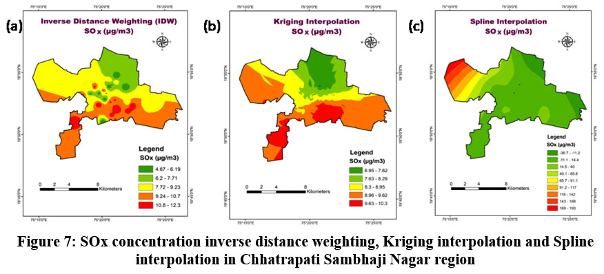Figure 7: SOx concentration inverse distance weighting, Kriging interpolation and Spline interpolation in Chhatrapati Sambhaji Nagar region Click here to view Figure

IDW map, Kriging map, and spline map of SOx concentration are presented in figure 7. The use of IDW for SOx concentration mapping, although effective for identifying localized hotspots, can result in overemphasis on specific monitoring stations. The IDW method displays SOx concentration ranging from 4.67 to 12.3 µg/m³. Higher concentrations are found primarily in the central and southern regions of Aurangabad, with hotspots around Kranti Chowk (12.27 µg/m³), Pundlik Nagar (11.66 µg/m³), and Kanchanwadi (11.95 µg/m³). The IDW map reflects localized high SOx concentrations near the monitoring stations. The influence of each station's data point is heavily reflected, leading to strong gradients near stations like Kranti Chowk and Pundlik Nagar. IDW tends to overemphasize the stations' influence, which can sometimes lead to overestimated concentrations near observation points. The highest concentration of SOx (over 10.8 µg/m³) is found in the central region of the city, extending from Akashwani Chowk to Kanchanwadi, as well as smaller patches in the southern areas.

The Kriging method revealed the concentration range of 6.95 to 10.3 µg/m³, providing a more balanced representation of air pollution in Aurangabad, which is slightly lower than the maximum concentration found in IDW. Kriging smoothens the data, leading to a more gradual change in SOx levels across the city. Kriging interpolation provides a more continuous and balanced representation of SOx distribution across the city, minimizing the sharp transitions found in the IDW method. Central and southern regions still exhibit higher SOx levels, but the transitions between high and low concentrations are more gradual and spread over larger areas. SOx concentrations are highest in the southern parts of the city, with values between 9.63 and 10.3 µg/m³. This covers areas like Kranti Chowk and Pundlik Nagar, though the concentration in other regions is lower than that shown in IDW.

The Spline method results in highly unrealistic values, with SOx concentrations ranging from -36.7 to 193 µg/m³. The presence of negative values, which are physically impossible for pollutant concentration, suggests that this method is inappropriate for this dataset. Spline interpolation exhibits extreme values and exaggerated variations across the city. While the central part of the city shows reasonable concentrations, the method introduces unusually high values in the western part of the city (even in areas without nearby observation points), which does not match the field data. Although some high SOx concentrations are visible in the central zone and southern parts of the city, the western areas show extremely high values (up to 193 µg/m³) that do not align with the field data, making this method unreliable for SOx mapping.

The Kriging method provides the most balanced and reliable interpolation for SOx concentrations. It smoothens the transitions between data points, leading to a more realistic spatial distribution without overemphasizing the influence of specific stations. The absence of extreme or unrealistic values makes Kriging the most appropriate method for this dataset. While IDW accurately reflects localized concentrations, it tends to overestimate SOx levels near the monitoring stations, leading to a more fragmented spatial distribution. The method is useful for identifying hotspots, but it may not be suitable for capturing overall trends in the region. The Spline method is not suitable for this dataset due to the unrealistic and erroneous values it generates. The presence of negative SOx concentrations and extreme highs in areas without observation data indicates poor model fit. Both IDW and Kriging show higher SOx concentrations in the central zone and southern parts of the city, particularly around Kranti Chowk, Pundlik Nagar, and Kanchanwadi. However, Kriging provides a smoother and more continuous spatial distribution, capturing broader trends more effectively. Spline introduces errors with unrealistic values in the western part of the city, where no monitoring stations are located, making its output unreliable. The IDW method shows the highest concentrations of SOx (up to 12.3 µg/m³), followed by Kriging (up to 10.3 µg/m³), while Spline generates implausible values (up to 193 µg/m³). This suggests that Kriging is the most reliable method, offering a more realistic assessment of SOx pollution distribution.

The IDW method shows NOx concentrations ranging from 2.51 to 21.8 µg/m³. The highest NOx concentrations are found in the central part of the city, particularly around the Maulana Azad College station (21.85 µg/m³), which is a hotspot. The IDW interpolation shows a clear influence of local monitoring stations. The highest values of NOx are concentrated in central locations, and the spatial distribution shows strong localized hotspots with sharp transitions between high and low concentrations. This results from the method’s emphasis on nearby data points. The highest concentrations are found around Maulana Azad College, Little Flower School, and City Chowk Police Station. These areas experience NOx concentrations exceeding 18 µg/m³, making them key hotspots for air pollution.

NOx Concentration: Kriging shows a similar concentration range, with values from 2.52 to 21.7 µg/m³. The concentration patterns are smoother compared to IDW, with a gradual transition between zones of high and low NOx levels. Kriging offers a more balanced spatial distribution, with smoother transitions between areas of varying concentrations. The Maulana Azad College region still stands out as a key hotspot for NOx pollution, but the spread of higher concentrations extends more evenly to surrounding areas, providing a more generalized view of NOx distribution across the city. Similar to IDW, the highest NOx concentrations are found around Maulana Azad College and the central part of the city. However, the Kriging method shows a more extended area of elevated NOx levels. NOx Concentration: The Spline method shows a much wider and unrealistic range of NOx concentrations, from -42.8 to 117 µg/m³. The presence of negative values makes this method inappropriate for air quality data, as it leads to physically impossible results. Spatial Distribution: The Spline interpolation map presents extreme values and sharp gradients that do not align with the field data. The highest NOx concentrations are in the north-western part of the city, far from known monitoring stations, indicating that this method is not capturing the true distribution of NOx pollution. The extreme and unrealistic concentrations shown by the Spline method, particularly in the northwest, are inconsistent with the field data and suggest that the method is not suitable for this analysis.

Kriging provides the most reliable interpolation method for this dataset, offering a smooth and balanced representation of NOx concentrations across the city. It reduces the influence of extreme values, leading to a more generalized yet accurate depiction of air pollution. IDW: IDW is effective for capturing localized hotspots of NOx pollution but may exaggerate the influence of individual stations, leading to sharper transitions and more isolated zones of high pollution.

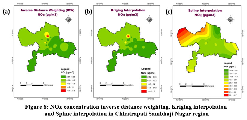Figure 8: NOx concentration inverse distance weighting, Kriging interpolation and Spline interpolation in Chhatrapati Sambhaji Nagar region Click here to view Figure

The Spline method produces unrealistic and erroneous values (including negative concentrations), making it unsuitable for air quality mapping in this case. Both IDW and Kriging show the highest NOx concentrations in the central part of Aurangabad, particularly around Maulana Azad College, Little Flower School, and City Chowk Police Station. Kriging provides a smoother transition, suggesting that high NOx levels are spread more evenly over a larger area, whereas IDW emphasizes more localized hotspots. Spline shows extreme values and patterns that do not align with real-world observations, making it unreliable for understanding the spatial trends of NOx pollution. The IDW method shows the highest NOx concentrations, reaching 21.8 µg/m³, while Kriging reaches up to 21.7 µg/m³, with a more generalized spread. Spline produces extreme and unrealistic values (up to 117 µg/m³), which are not consistent with the actual data. IDW maps, Kriging map, Spline map for NOx concentration arepresented in figure 8.

IDW has been commonly used in air pollution studies to provide an interpolated surface based on localized ground measurements.⁵⁹ The IDW map shows a concentration of PM10 values ranging from 40.3 to 211 µg/m³. IDW tends to overemphasize nearby measurements, creating sharp transitions between zones. The highest PM10 concentration is observed in the central zone and southern parts of the city, particularly around the Akashwani Chowk and Kranti Chowk stations, where levels exceed 178 µg/m³. IDW emphasizes the influence of nearby points more strongly, leading to a high concentration of PM10 around specific monitoring stations (like Kranti Chowk). However, the interpolation method shows fewer smooth transitions between zones, as it directly reflects the influence of nearby points. Central and south-central parts of the city show the highest PM10 values, with a hotspot around the Kranti Chowk region.

PM10 Concentration: Kriging is well-regarded for its ability to generate smoother and more continuous spatial distributions.⁶⁰ The Kriging map displays a PM10 concentration ranging from 80.1 to 120 µg/m³, which seems lower than the IDW results. The spatial distribution is more uniform, with gradual transitions between different zones.The method is especially useful in minimizing the effect of extreme values, leading to a more generalized, reliable estimate. Kriging is more advanced in estimating values in areas with no data points, making it useful for capturing the general trend across the city. It reduces the influence of extreme values observed in IDW and provides a smoother, more continuous representation of PM10 dispersion. The highest PM10 concentrations are found in the central city area, with a smoother transition to lower values in the northern and southern parts. The Akashwani Chowk and Kranti Chowk areas again stand out as pollution hotspots, but the overall spread of high PM10 values extends further.

The Spline method presents an unusual result, with PM10 values ranging from -365 to 1140 µg/m³. The negative values are physically unrealistic and suggest that the Spline interpolation is not appropriate for this dataset. Spline interpolation, although occasionally used for environmental data, can result in physically unrealistic values when applied to air quality data. Spatial Distribution: Spline interpolation appears to create exaggerated fluctuations in PM10 values, especially in areas without nearby data points, leading to unrealistic gradients. The high concentration zone in the northern parts of the map is inconsistent with the monitoring station data, indicating this method's poor fit for this dataset. Despite the errors, high PM10 levels are still concentrated in the central parts of the city, particularly around Akashwani Chowk and Kranti Chowk. However, the extreme values seen in the north do not align with the field data and suggest inaccuracies in the method's output.

The Kriging method provides the most reliable spatial distribution of PM10 levels due to its ability to minimize the effect of extreme values while ensuring a smooth, continuous representation of the data. It balances interpolation accuracy and realistic representation, making it the most suitable method for PM10 mapping in this case. While IDW effectively captures localized hotspots around monitoring stations, it may overemphasize the impact of individual stations, leading to sharp transitions between zones. It is useful for a more localized assessment but may not capture the broader trends as effectively as Kriging. The unrealistic values (negative PM10 concentrations and extreme highs) generated by the Spline method indicate that it is not a suitable method for this dataset. The spline's tendency to create unrealistic fluctuations makes it less reliable for air quality assessments like PM10 mapping.

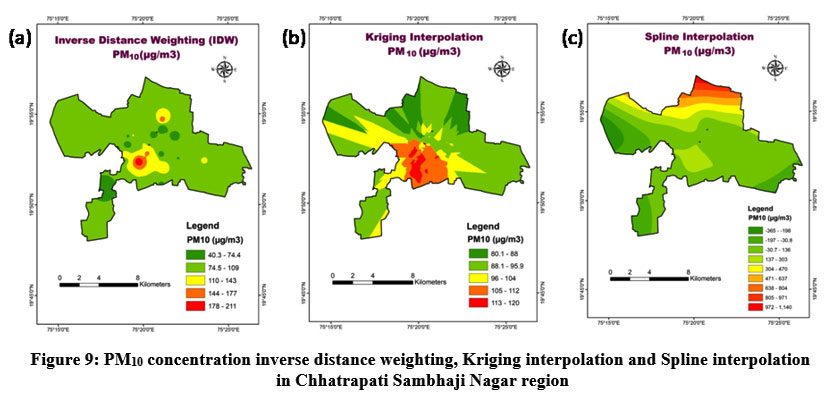Figure 9: PM10 concentration inverse distance weighting, Kriging interpolation and Spline interpolation in Chhatrapati Sambhaji Nagar region Click here to view Figure

Both IDW and Kriging identify central regions (Akashwani Chowk and Kranti Chowk) as areas of concern with higher PM10 concentrations. Kriging offers a smoother transition and indicates a broader spread of pollution, while IDW creates more localized hotspots. Spline, while consistent in showing concentrations high in the central zone of the city, presents errors and unrealistic values, making its results unreliable. The IDW method shows the highest PM10 concentrations (up to 211 µg/m³), followed by Kriging (up to 120 µg/m³), and Spline presents implausibly high values (up to 1140 µg/m³). This suggests that Kriging offers a more balanced and realistic assessment of PM10 distribution, while IDW may overestimate concentrations around specific points.IDW map, Kriging map, spline map of PM10 concentration are presented in figure 9.

The IDW method revealed the PM 2.5 concentrations ranging from 7.11 to 280 µg/m³. The highest concentrations are noted around Sutgirni Chowk (280 µg/m³) and Shivaji Chowk, Shivaji Nagar (260 µg/m³), reflecting high pollution levels in these areas. Spatial Distribution method emphasizes the influence of individual monitoring stations, leading to localized high-concentration areas. This can result in sharp transitions between zones of high and low concentrations, particularly evident near major roads and industrial areas. The highest PM2.5 concentrations are in the central and south-western parts of the city, highlighting these regions as major hotspots for air pollution. PM2.5 Concentration: Kriging results show a more balanced distribution, with concentrations ranging from 13.1 to 244 µg/m³. This method smoothens the extreme values seen in IDW, providing a more continuous spatial distribution. Kriging offers a smoothed overview, reducing the impact of isolated high readings and providing a more uniform pollution map. The gradients between high and low concentrations are more gradual, indicating a broader area of influence for each station. The central regions, especially around Shivaji Chowk and Sutgirni Chowk, still exhibit higher PM2.5 levels but the transition between different concentration zones is less abrupt compared to IDW.

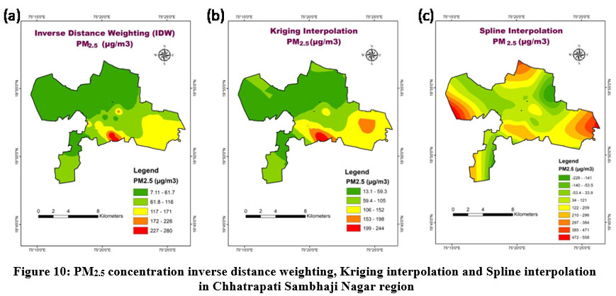Figure 10: PM2.5 concentration inverse distance weighting, Kriging interpolation and Spline interpolation in Chhatrapati Sambhaji Nagar region Click here to view Figure

The Spline method displays a broad range of concentrations, from -228 to 558 µg/m³. This method produces some unrealistic negative values, indicating that it may not be appropriate for this dataset. Spatial Distribution: Spline creates a smooth gradient across the city but tends to exaggerate the concentration extremes, particularly on the edges of the map where no data points exist. This method seems to interpolate beyond realistic bounds, suggesting less reliability for this type of environmental data. Despite generating some extreme and unrealistic values, high concentrations are again noticed in central Aurangabad, with exaggerated peaks compared to actual monitoring data. IDW map, Kriging map, Spline map for PM 2.5 concentration are presented in figure.10

Kriging provided a balanced and realistic assessment of PM2.5 distribution, smoothing out the anomalies and providing a map that likely better reflects the average air quality conditions across the city. While effective at highlighting specific hotspots, it might overemphasize the pollution levels directly around the monitoring stations, potentially skewing public perception and policy focus. The splineapproach was not suitable for this dataset as it introduces unrealistic extremes, making it unreliable for practical air quality assessment and management. Both IDW and Kriging identify central Aurangabad as a significant concern for PM2.5 pollution, with specific attention needed on the areas around major traffic junctions and industrial zones. Spline exaggerates the spatial extent and severity of pollution, which could mislead decision-making processes related to air quality management. IDW method shows the highest pollution levels but may not accurately represent the broader city-wide air quality. Kriging suggests high levels but with a more moderate max value, potentially offering a more accurate picture of widespread pollution levels. Spline provides an exaggerated perspective, with both the lowest and highest extremes, highlighting its unsuitability.

Conclusions

In this experimental study,we employed in situ and satellite data collection for two years to investigate major pollutants in the Northwest region of Marathwada. The findings revealed an annual increase in pollutant levels, with ambient air quality parameters alarmingly close to, if not exceeding, the permissible limits of NAAQ standards. Statistical correlation analysis validated the integration of remote sensing technologies with ground-based measurements for effective air quality monitoring. The negligible difference in pollutant levels between residential and industrial areas suggested significant contributions from traffic emissions, local commercial activities, construction or demolition activities, waste management failures, and regional atmospheric conditions. This underscores the need for comprehensive air quality management strategies that address multiple pollution sources beyond industrial activities.Anthropogenic activities, including ever-increasing industrialization, urbanization, and vehicular pollution, negatively impact environmental pollution concentrations. A significant dependency of air pollutants on meteorological factors was also recorded. The economic and health implications of air pollution are alarming, necessitating a strategic plan with mitigation strategies to promote sustainability.

Acknowledgment

All the authors wish to thanks to Shri A.N.Kadam.Chancellor, MGM University University, Chh.Sambhajinagar(MS).

Funding Sources

The author(s) received no financial support for the research, authorship, and/or publication of this article.

Conflict of Interest

The authors do not have any conflict of interest.

Data Availability Statement

The manuscript incorporates all datasets produced or examined throughout this research study.

Ethics Statement

This research did not involve human participants, animal subjects, or any material that requires ethical approval.

Informed Consent Statement

This study did not involve human participants, and therefore, informed consent was not required.

Author Contributions

R V Wanjule: Performed the experiments and has written original draft,

Dr.Mrs.M.N.Mangulkar: Extended her supervision and reviewing of this manuscript.

References

1. Kaushik G, Khalid MA, Mumtaz N, Izhar T. Perceptions of School Students Regarding Air Pollution: A Study of Aurangabad City in Maharashtra, India. In: Hussain CM, ed. Handbook of Environmental Materials Management. Springer International Publishing; 2020:1-24. doi:10.1007/978-3-319-58538-3_237-1
   CrossRef
2. Jogdand O, Bandela NN, Kaushik G, Chel A. Determination of Select Heavy Metals in Air Samples from Aurangabad City. In: Hussain CM, ed. Handbook of Environmental Materials Management. Springer International Publishing; 2018:1-10. doi:10.1007/978-3-319-58538-3_164-1
   CrossRef
3. Kaushik G, Patil S, Chel A. Air Quality Status and Management in Tier II and III Indian Cities: A Case Study of Aurangabad City, Maharashtra. In: Hussain CM, ed. Handbook of Environmental Materials Management. Springer International Publishing; 2018:1-22. doi:10.1007/978-3-319-58538-3_156-1
   CrossRef
4. Robert Hijmans. GADM. Global Administrative Areas Database Management. December 23, 2024. Accessed December 23, 2024. https://gadm.org/maps/IND.html
5. Maharashtra Pollution Control Board. Air Quality Status of Maharashtra 2019-2020 Accessed on 4 June 2024.; 2020. https://www.mpcb.gov.in/sites/default/files/air-quality/AIRQualityReport 2019202210 2020.pdf
6. Sahani N. Assessment of spatio-temporal changes of land surface temperature (LST) in Kanchenjunga Biosphere Reserve (KBR), India using Landsat satellite image and single channel algorithm. Remote Sensing Applications: Society and Environment. 2021;24:100659. doi:10.1016/j.rsase.2021.100659
   CrossRef
7. Lemenkova P, Debeir O. Satellite Image Processing by Python and R Using Landsat 9 OLI/TIRS and SRTM DEM Data on Côte d’Ivoire, West Africa. Journal of Imaging. 2022;8(12):317. doi:10.3390/jimaging 8120317
   CrossRef
8. Ghosh S, Das A, Hembram TK, Saha S, Pradhan B, Alamri AM. Impact of COVID-19 Induced Lockdown on Environmental Quality in Four Indian Megacities Using Landsat 8 OLI and TIRS-Derived Data and Mamdani Fuzzy Logic Modelling Approach. Sustainability. 2020;12(13):5464. doi:10.3390/su12135464
   CrossRef
9. Nazeer M, Ilori CO, Bilal M, et al. Evaluation of atmospheric correction methods for low to high resolutions satellite remote sensing data. Atmospheric Research. 2021;249:105308. doi:10.1016/j.atmosres. 2020.105308
   CrossRef
10. Dong P, Gao L, Zhan W, et al. Global comparison of diverse scaling factors and regression models for downscaling Landsat-8 thermal data. ISPRS Journal of Photogrammetry and Remote Sensing. 2020;169:44-56. doi:10.1016/j.isprsjprs.2020.08.018
    CrossRef
11. Zhai Y, Roy DP, Martins VS, Zhang HK, Yan L, Li Z. Conterminous United States Landsat-8 top of atmosphere and surface reflectance tasseled cap transformation coefficients. Remote Sensing of Environment. 2022;274:112992. doi:10.1016/j.rse.2022.112992
    CrossRef
12. Wang W, Li S, Hashimoto H, et al. An Introduction to the Geostationary-NASA Earth Exchange (GeoNEX) Products: 1. Top-of-Atmosphere Reflectance and Brightness Temperature. Remote Sensing. 2020;12(8):1267. doi:10.3390/rs12081267
    CrossRef
13. Sun B, Schäfer M, Ehrlich A, Jäkel E, Wendisch M. Influence of atmospheric adjacency effect on top-of-atmosphere radiances and its correction in the retrieval of Lambertian surface reflectivity based on three-dimensional radiative transfer. Remote Sensing of Environment. 2021;263:112543. doi:10.1016/j.rse.2021.112543
    CrossRef
14. Moran MS, Jackson RD, Slater PN, Teillet PM. Evaluation of simplified procedures for retrieval of land surface reflectance factors from satellite sensor output. Remote Sensing of Environment. 1992;41(2):169-184. doi:10.1016/0034-4257(92)90076-V
    CrossRef
15. Moran MS, Bryant R, Holifield CD, McElroy S. Refined empirical line approach for retrieving surface reflectance from EO-1 ALI images. IEEE Transactions on Geoscience and Remote Sensing. 2003;41(6):1411-1414. doi:10.1109/TGRS.2003.813207
    CrossRef
16. Cui L, Li G, Ren H, et al. Assessment of atmospheric correction methods for historical Landsat TM images in the coastal zone: A case study in Jiangsu, China. European Journal of Remote Sensing. 2014;47(1):701-716. doi:10.5721/EuJRS20144740
    CrossRef
17. Ding H, Shi J, Wang Y, Wei L. An improved dark-object subtraction technique for atmospheric correction of Landsat 8. In: Ninth International Symposium on Multispectral Image Processing and Pattern Recognition. ; 2015. doi:https://doi.org/10.1117/12.2205567
    CrossRef
18. Halder B, Ahmadianfar I, Heddam S, et al. Machine learning-based country-level annual air pollutants exploration using Sentinel-5P and Google Earth Engine. Scientific Reports. 2023;13(1):7968. doi:10.1038/s41598-023-34774-9
    CrossRef
19. Manning N, Li Y, Liu J. Broader applicability of the metacoupling framework than Tobler’s first law of geography for global sustainability: A systematic review. Geography and Sustainability. 2023;4(1):6-18. doi:10.1016/j.geosus.2022.11.003
    CrossRef
20. Auscher P, Portal P. Stochastic and deterministic parabolic equations with bounded measurable coefficients in space and time: Well-posedness and maximal regularity. Journal of Differential Equations. 2025;420:1-51. doi:10.1016/j.jde.2024.11.038
    CrossRef
21. Lu GY, Wong DW. An adaptive inverse-distance weighting spatial interpolation technique. Computers & Geosciences. 2008;34(9):1044-1055. doi:10.1016/j.cageo.2007.07.010
    CrossRef
22. Ravi Gupta. Remote Sensing Geology.; 2018. Accessed December 3, 2024. https://link.springer.com/book/10.1007/978-3-662-55876-8
23. Miao C, Wang Y. Interpolation of non-stationary geo-data using Kriging with sparse representation of covariance function. Computers and Geotechnics. 2024;169:106183. doi:10.1016/j.compgeo.2024.106183
    CrossRef
24. Hu M, Li H, Lu J, Zou H, Ma Q. An online modeling virtual sensing technique based on kriging interpolation for active noise control. Mechanical Systems and Signal Processing. 2025;224:112186. doi:10.1016/j.ymssp.2024.112186
    CrossRef
25. Li L, Jiang Z, Duan N, Dong W, Hu K, Sun W. An Approach to Optimize Police Patrol Activities Based on the Spatial Pattern of Crime Hotspots1. In: Xiong G, Liu Z, Liu XW, Zhu F, Shen D, eds. Service Science, Management, and Engineering:. Academic Press; 2012:141-163. doi:10.1016/B978-0-12-397037-4.00008-9
    CrossRef
26. Haining R, Law J, Griffith D. Modelling small area counts in the presence of overdispersion and spatial autocorrelation. Computational Statistics & Data Analysis. 2009;53(8):2923-2937. doi:10.1016/j.csda. 2008.08.014
    CrossRef
27. Muhamad Ali MZMA, Othman F. Selection of variogram model for spatial rainfall mapping using Analytical Hierarchy Procedure (AHP). Scientia Iranica. Published online February 1, 2017. doi:10.24200/ sci.2017.2374
    CrossRef
28. de Carvalho PRM, da Costa JFCL. Automatic variogram model fitting of a variogram map based on the Fourier integral method. Computers & Geosciences. 2021;156:104891. doi:10.1016/j.cageo.2021.104891
    CrossRef
29. Xu J, Zhang L, Wang Y, Wang C, Zheng J, Yu Y. Probabilistic estimation of cross-variogram based on Bayesian inference. Engineering Geology. 2020;277:105813. doi:10.1016/j.enggeo.2020.105813
    CrossRef
30. Gräler B, Pebesma E, Heuvelink G. Spatio-Temporal Interpolation using gstat. 2016;8(8):204-218. doi:https://doi.org/10.32614/RJ-2016-014
    CrossRef
31. Larsson DGJ. Pollution from drug manufacturing: review and perspectives. Philosophical Transactions of the Royal Society B: Biological Sciences. 2014;369(1656):20130571. doi:10.1098/rstb.2013.0571
    CrossRef
32. Lin Q, Gao Z, Zhu W, Chen J, An T. Underestimated contribution of fugitive emission to VOCs in pharmaceutical industry based on pollution characteristics, odorous activity and health risk assessment. Journal of Environmental Sciences. 2023;126:722-733. doi:10.1016/j.jes.2022.03.005
    CrossRef
33. Pfeffer MA, Arellano S, Barsotti S, et al. SO2 emission rates and incorporation into the air pollution dispersion forecast during the 2021 eruption of Fagradalsfjall, Iceland. Journal of Volcanology and Geothermal Research. 2024;449:108064. doi:10.1016/j.jvolgeores.2024.108064
    CrossRef
34. Wang Y, Eriksson T, Luo N. The health impacts of two policies regulating SO2 air pollution: Evidence from China. China Economic Review. 2023;78:101937. doi:10.1016/j.chieco.2023.101937
    CrossRef
35. Kannan K. Preparation of Eco-bricks with a topical coating of silver nanoparticles. Materials Today: Proceedings. Published online July 1, 2023. doi:10.1016/j.matpr.2023.06.285
    CrossRef
36. Shi C, Zhang Z, Xiong S, et al. Harmonizing atmospheric ozone column concentrations over the Tibetan Plateau from 2005 to 2022 using OMI and Sentinel-5P TROPOMI: A deep learning approach. International Journal of Applied Earth Observation and Geoinformation. 2024;129:103808. doi:10.1016/j.jag.2024.103808
    CrossRef
37. Government of India. Location Specific Weather Forecast, India meteorological department. 2023. Accessed June 20, 2024. https://internal.imd.gov.in/pages/city_weather_main_mausam.php
38. Polemiti E, Hese S, Schepanski K, Yuan J, Schumann G, environMENTAL consortium. How does the macroenvironment influence brain and behaviour—a review of current status and future perspectives | Molecular Psychiatry. Molecular Psychiatry. Published online April 24, 2024. doi:10.1038/s41380-024-02557-x
    CrossRef
39. Shen Y, Jiang F, Feng S, et al. Increased diurnal difference of NO2 concentrations and its impact on recent ozone pollution in eastern China in summer. Science of The Total Environment. 2023;858:159767. doi:10.1016/j.scitotenv.2022.159767
    CrossRef
40. Jurado X, Reiminger N, Vazquez J, et al. Assessment of mean annual NO2 concentration based on a partial dataset. Atmospheric Environment. 2020;221:117087. doi:10.1016/j.atmosenv.2019.117087
    CrossRef
41. Mar? M, Bielawska M, Simeonov V, Namie?nik J, Zabiega?a B. The effect of anthropogenic activity on BTEX, NO2, SO2, and CO concentrations in urban air of the spa city of Sopot and medium-industrialized city of Tczew located in North Poland. Environmental Research. 2016;147:513-524. doi:10.1016/j.envres.2016.03.014
    CrossRef
42. Tian XP, Wang D, Wang YQ, et al. Long-term variations and trends of tropospheric and ground-level NO2 over typical coastal areas. Ecological Indicators. 2024;164:112163. doi:10.1016/j.ecolind.2024.112163
    CrossRef
43. Jion MostMMF, Jannat JN, Mia MdY, et al. A critical review and prospect of NO2 and SO2 pollution over Asia: Hotspots, trends, and sources. Science of The Total Environment. 2023;876:162851. doi:10.1016/j.scitotenv.2023.162851
    CrossRef
44. Huang Z, Xu X, Ma M, Shen J. Assessment of NO2 population exposure from 2005 to 2020 in China. Environmental Science and Pollution Research. 2022;29(53):80257-80271. doi:10.1007/s11356-022-21420-6
    CrossRef
45. Chi Y, Fan M, Zhao C, et al. Ground-level NO2 concentration estimation based on OMI tropospheric NO2 and its spatiotemporal characteristics in typical regions of China. Atmospheric Research. 2021;264:105821. doi:10.1016/j.atmosres.2021.105821
    CrossRef
46. Zheng, Yang, Wu, Marinello. Spatial Variation of NO2 and Its Impact Factors in China: An Application of Sentinel-5P Products. Remote Sensing. 2019;11(16):1939. doi:10.3390/rs11161939
    CrossRef
47. Schneider P, Hamer PD, Kylling A, Shetty S, Stebel K. Spatiotemporal Patterns in Data Availability of the Sentinel-5P NO2 Product over Urban Areas in Norway. Remote Sensing. 2021;13(11):2095. doi:10.3390/ rs13112095
    CrossRef
48. Lee HW, Kang SC, Kim SY, Cho YJ, Hwang S. Long-term Exposure to PM10 Increases Lung Cancer Risks: A Cohort Analysis. Cancer Res Treat. 2022;54(4):1030-1037. doi:10.4143/crt.2021.1030
    CrossRef
49. Lee YM, Lee JH, Kim HC, Ha E. Effects of PM10 on mortality in pure COPD and asthma-COPD overlap: difference in exposure duration, gender, and smoking status | Scientific Reports. Scientific Reports. 2020;10(1):2402. doi:10.1038/s41598-020-59246-2
    CrossRef
50. Medina-Ramón M, Zanobetti A, Schwartz J. The effect of ozone and PM10 on hospital admissions for pneumonia and chronic obstructive pulmonary disease: a national multicity study. Am J Epidemiol. 2006;163(6):579-588. doi:10.1093/aje/kwj078
    CrossRef
51. Gaio V, Roquette R, Monteiro A, Ferreira J, Matias Dias C, Nunes B. Investigating the association between ambient particulate matter (PM10) exposure and blood pressure values: Results from the link between the Portuguese Health Examination Survey and air quality data. Revista Portuguesa de Cardiologia. 2023;42(3):251-258. doi:10.1016/j.repc.2022.02.011
    CrossRef
52. Lee JH, Byun MS, Yi D, et al. Long-Term Exposure to PM10 and in vivo Alzheimer’s Disease Pathologies. JAD. 2020;78(2):745-756. doi:10.3233/JAD-200694
    CrossRef
53. Liu R, Young MT, Chen JC, Kaufman JD, Chen H. Ambient Air Pollution Exposures and Risk of Parkinson Disease. Environ Health Perspect. 2016;124(11):1759-1765. doi:10.1289/EHP135
    CrossRef
54. Mushtaq Z, Bangotra P, Gautam AS, et al. Satellite or ground-based measurements for air pollutants (PM2.5, PM10, SO2, NO2, O3) data and their health hazards: which is most accurate and why? Environ Monit Assess. 2024;196(4):342. doi:10.1007/s10661-024-12462-z
    CrossRef
55. Chauhan PK, Kumar A, Pratap V, Singh AK. Seasonal characteristics of PM1, PM2.5, and PM10 over Varanasi during 2019–2020. Front Sustain Cities. 2022;4:909351. doi:10.3389/frsc.2022.909351
    CrossRef
56. Elbayoumi M, Ramli NA, Md Yusof NFF, Al Madhoun W. Spatial and seasonal variation of particulate matter (PM10 and PM2.5) in Middle Eastern classrooms. Atmospheric Environment. 2013;80:389-397. doi:10.1016/j.atmosenv.2013.07.067
    CrossRef
57. Kim SU, Kim KY. Physical and chemical mechanisms of the daily-to-seasonal variation of PM10 in Korea. Science of The Total Environment. 2020;712:136429. doi:10.1016/j.scitotenv.2019.136429
    CrossRef
58. Kim HC, Kim S, Kim BU, et al. Recent increase of surface particulate matter concentrations in the Seoul Metropolitan Area, Korea | Scientific Reports. Scientific Reports. 2017;7(1):4710. doi:10.1038/s41598-017-05092-8
    CrossRef
59. Sajjadi SA, Zolfaghari G, Adab H, Allahabadi A, Delsouz M. Measurement and modeling of particulate matter concentrations: Applying spatial analysis and regression techniques to assess air quality. MethodsX. 2017;4:372-390. doi:10.1016/j.mex.2017.09.006
    CrossRef
60. Li J, Heap AD. Spatial interpolation methods applied in the environmental sciences: A review. Environmental Modelling & Software. 2014;53:173-189. doi:10.1016/j.envsoft.2013.12.008
    CrossRef
61. Nadzri Othman,Mohd Zubir Mat Jafri & Lim Hwee San (2010), “Estimating Particulate Matter Concentration over Arid Region Using Satellite Remote Sensing: A Case Study in Makkah, Saudi Arabia” Modern Applied Science,4,pp.131-142.
    CrossRef
62. Chander, G., Markham, B.L. and Helder, D.L.,( 2009).” Summary of current radiometric calibration coefficients for Landsat MSS, TM, ETM+, and EO-1 ALI sensors”. Remote sensing of environment, 113(5), pp.893-903.Chander, G., Markham, B.L. and Helder, D.L.,( 2009).” Summary of current radiometric calibration coefficients for Landsat MSS, TM, ETM+, and EO-1 ALI sensors”. Remote sensing of environment, 113(5), pp.893-903.
    CrossRef