Current World Environment

Introduction

Flood quantity is used in design of hydraulic structures, which are affected by hydrological events considering factors such as structural safety, lifetime and probable damage. This quantity is also called design flood. Calculating design flood for large dams is considered as one of the most important steps in dam engineering studies. Comparing the damages resulting from dam failure with the profits gained by constructing them and their optimize utilization shows the high sensitivity of selecting design flood in order to maintain stability of dams. Several methods were proposed to compute the design flood. The most important methods are frequency analysis, regional analysis, rainfall-runoff models, empirical relationships, flood envelope curve and using historical floods.

 One of the most common causes of dam failure is considered as overtopping occurred due to a flood larger than mitigation capacity of the reservoir and spillway discharge. Several reports suggested that 41% of dam failure accidents are caused by low capacity of dam’s spillway(Bouvard 1988).³ Numerous other reports and articles reported the risk of dam failure due to the flyover at least as 30%; moreover, often 30 to 40 percent of total reported dam failures are due to the flyover (Hagen 1982).⁷ Overall, 40 incidents among 100 dam failures from 1950 to 1990 were due to the dam overtop (ICOLD 1997).¹³

Statistics and information of the recorded maximum floods in a dam construction site play a decisive role in design flood estimation. Meanwhile, before making any form of calculations, we should be confident about the accuracy of information, we should closely determine weight and value of each recorded quantity - as real dimensions within the desired time span - and specify its position as much as possible. However, unfortunately, value and position of registration statistics are forgotten in some cases; all pieces of information are given an equal value and floods with different return periods are calculated using common techniques. As a result, the obtained figures (design floods) have no consistency with the case study watershed and the costs borne to construct massive concrete structures for the floods can be resembled in the fortune premium that should be paid for the fictitious and imaginary accidents.  

Observed data can significantly affect the design estimates. The current study aims at determining the role of outlier date in estimating design flood. In this regard, flood estimate using flood frequency analysis is carried out once over complete data series, and the other time on the series with deleted outlier. Then by combining outlier data with other systematic data and revising the statistical distribution parameters from the selected distribution, flood magnitudes corresponding to various return periods are compared.  

Materials and Methods

Case Study

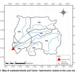
Tamer watershed with approximately 1531 square kilometer in area is located in the southeastern part of the Caspian Sea coastline in Iran. It is one of the main sub water sheds of Golestan watershed. This area is located between 55°30’ and 56°4’ E longitude and 37°,24’  to 37°,48’ N latitude. Figure 1 shows the map of Tamer subwatersheds and its drainage network.

Figure 1: Map of subwatersheds and Tamer hydrometric station in the case study region Click here to View figure

Outlier data

Outlier data are single data points that appear to depart significantly from the trend of the other data. They are usually divided into three groups: 1) Observation made by collection error and/or data registration 2) Observations made by natural factors 3) Observations made by unnatural factors such as dam failure (Transportation 2004).¹⁶ Both high outlier floods and historical floods are considered as exceptional large floods, the former was observed during the period of systematic registration, and the latter were observed out of this period. The systematic record can be used directly in flood frequency analysis. The non-systematic records cannot be used unless additional information can be supplied to relate them to the population of all flood peaks (IACWD 1982).¹¹

According to the proposal given by Water Resources Association of America in 1982, if the coefficient of skewness of data is greater than 0.4, outlier tests for large values should be conducted. If the coefficient of skewness of the data is less than -0.4 outlier tests should be conducted for small values, if the coefficient of skewness is between -0.4 and 0.4, outlier tests should be conducted for both large and small values (IACWD 1982).¹¹ Although many methods have already been proposed to detect outlier data, none of them are universally accepted (Garcia 2012).⁴

 In the case of peak flows which are considered as outlier data, required tests should be performed to avoid probable errors in the first calculations on statistical sheets due to transferring data to different forms or in computer. Then, the former data is compared with historical data or data from adjacent area. According to the Water Resources Association of America, if the available data shows that an outlier data can be accepted as maximum data in a long time, it can be taken into account as historical data. Data which are below the lower threshold should be eliminated from data set of maximum flow values. Then the appropriate distribution is selected based on remaining data (IACWD 1982).¹¹

Flood frequency analysis

Flood frequency analysis is an important tool for design of installations such as dams, bridges, culverts, and water supply systems and flood control structures. This includes most part of research activities in the field of statistics and probability in hydrology. The small and large scale of a hydraulic structure as well as construction cost in a hydro project has a direct relationship with selecting the desired flood. If the selected flood was larger than average, the constructed structure would be larger, more tremendous and stronger. As a result, construction cost will increase. The main objective of flood frequency analysis lies in obtaining return periods of measurable events (probability of occurrence of the events) and estimating the magnitude of an event for a specified return period usually larger than the length of recorded events(Hamed and Rao 1999⁷; Kite 1977¹³). Estimating flood flow rate and return periods of scarce events such as floods and severe rainfalls at some hydraulic structures are considered as one of the most important design factors (Hosking and Wallis 1993).⁹

One of the most important factors in frequency analysis lies in availability of the long and accurate data series. Hosking and Wallis (1993),¹⁰ Singh (1998),¹⁵ Hamed and Rao (1999),⁷ Griffis and Stedinger (2007)⁵ thoroughly studied flood frequency analysis and emphasized that probability of occurrence of a severe flood is an extrapolation based on limited data and short length of data series or missing data causes considerable uncertainties in extrapolation of flood using conventional statistical methods. Estimates derived from small sample flood data may be associated with unreasonable or unrealistic factors.

Normal function, the two-parameters log-normal, three-parameters log-normal, Pearson Type III, Log-Pearson Type III (LP-III), two-parameters gamma and gumbel are the most widely used continuous probability distribution functions used in flood frequency analysis to find the magnitude of a flood event corresponds to a specific return period, i.e. a probability of occurrence. The integral of probability distribution function (PDF) yields the cumulative distribution function (CDF). 

Parameters of statistical distributions are calculated from available data using some methods such as method of moments (MOM) and maximum likelihood method (MLM). Method of moments is relatively simple. However, the results are less accurate, especially if the number of data is small. Parameters of a probability distribution function are estimated by equating the sample moments (m) to probability distribution function moments. The maximum likelihood method is more accurate. However, it is very time-consuming and complicated (Hamed and Rao 1999).⁷

A set of goodness of fit tests such as Kolmogorov-Smirnov and Chi-square were used in order to judge about the degree of fitness of probability distribution models with observed data. If the fit was quite acceptable, the distribution would be selected for further analyses. Acceptable distributions were ranked based on two statistics, namely mean relative deviation (MRD) and mean square relative deviation (MSRD) which are explained in Equations 1 and 2. The distribution with the smallest MRD and MSRD has the best fit on observed data.

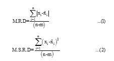
where x_i represents the i^th observed data,  denotes the estimated value of x_i, n represents number of data and m denotes number of parameters of the distribution (Adeyemo and Olofintoye 2014)¹.

Integrating outlier data with systematic data

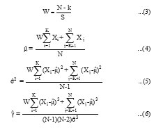
In order to integrate above outlier data with either historical flood data or the rest of systematic data, the method proposed by United States Water Resources Committee was applied to modify parameters of the statistical distributions, e.g. mean, variance and coefficient of skewness. These modifications without following outlier data is performed using Equations 3 to 6

Empirical likelihood of the points, p(i) is modified using weibull relation as follows:

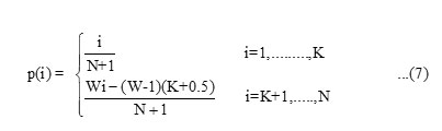
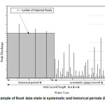
where w represents the weight factor, H denotes historical or exceptional flood record period (year), S represents the systematic data recording period (year), N denotes total data recording period with respect to years (N= S+H) , k represents the number of historical floods, x denotes the log of flow rate data,  represents the

modified mean, δ² denotes the modified variance and represents modified coefficient of skewness. In Figure 2, an example of a flood data state is shown in both systematic and historical periods (England Jr et al. 2003).³

Figure 2: An example of flood data state in systematic and historical periods (England et al., 2003) Click here to View figure

Results and Discussion

In this study, annual momentary maximum flow rates at Tamer hydrometric station located at outlet area of the region under study was studied. The station was located at coordinates 59^◦29^/30^// eastern longitude and 37^◦28^/30^// northern latitude at 132 meters above sea level. Figure 3 shows changes in the values ​​of maximum momentary flow rates in Tamer hydrometric station during statistical years.

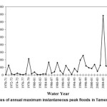Figure 3: Time series of annual maximum instantaneous peak floods in Tamer hydrometric station  Click here to View figure

According to outliers test results ​and the relatively large difference between the maximum observed flow (783 m³/s from 2004 to 2005) and the next highest flow (230 m³/s from 2007 to 2008) with a ratio about 3.4, the maximum flow rate at the given station was considered as outlier data (Heidarpour et al., 2015).⁸ Table 1 contains the statistical properties of annual momentary maximum flood data in hydrometric station for both normal and natural logarithmic values considering complete series and after removal of outlier data.

Table 1: statistical properties of annual maximum flood data in Tamer hydrometric station

Figure 4: Changes in 1000- and 10000-yr return period flood magnitudes vs. outlier return periods Click here to View figure

Effect of involving outlier data in flood frequency analysis

In flood frequency analysis, first frequency of annual instantaneous maximum floods was analyzed using the complete data series. Next, flood frequency analysis was performed by removing the outliers to understand the role of outliers in estimating design floods with different return periods. To exam data quality, some statistical tests were applied to check randomness, existence of trend, data independency and homogeneity using Consolidated Frequency Analysis (CFA) Software (Pilon and Harvey 1994).¹⁴ Then, hydrological frequency analysis software (HYFA) was used for flood frequency analysis. The software fits data with seven frequency distribution functions. Then, parameters of probability distributions were estimated using the method of moments and maximum likelihood approach. The parameters were calculated at different return periods. Then, the appropriate distribution was determined using goodness-of-fit Chi-square test and mean relative deviation (MRD) and mean square relative deviation (MSRD) (Hemmadi et al., 2007).⁹

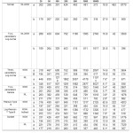Table 2: Estimated floods of different return periods in complete series and after removing outlier data (discharge in m3/s) Click here to View table

Figure 5: Observed and estimated floods corresponding to different return periods with 95% confidence intervals at Tamer hydrometric station Click here to View figure

Table 3 contains the results of frequency analysis with different return periods for annual instantaneous maximum flow at Tamer hydrometric station. According to these results, LP-III distribution has the lowest value of mean relative deviation (MRD) and mean square relative deviation (MSRD), and hence it was selected as the best probability distribution among other distributions accepted in Chi-square goodness-of-fit test.

Table 3: Sensitivity analysis of outlier data for different return periods (Discharge m³/s)

Based on the results, it can also be argued that although outlier did not change type of the selected statistical distribution, but it affected flood estimation results, especially in different return periods. Then, if observed outlier data was given the same value as other flood data at Tamer hydrometric station, instantaneous maximum flood with the 10000-year return period will be estimated as 3320 m³/s using the LP-III distribution. If the outlier was removed, then the 10000-year flood value will be reduced to 1340 m³/s (approximately 60% decrease).  

Results of merging outlier data with systematic data in frequency analysis

HEC-SSP version 2.0 statistical software developed by United States Army Corps of Engineers was used to integrate outlier data with remaining systematic data in frequency analysis. The original and trial versions of this software were offered in 2006. Based on B17 Bulletin of Water Resources Committee of the United States, this software can be used for statistical analyses of hydrological data. The new version of the software presented in 2010 was used in this study. Some features were added to this version such as flood flow and rainfall frequency analysis, daily flow volume frequency analysis, duration analysis, analysis of the charts combined by two separate sources (USACE 2010).¹⁷

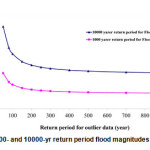
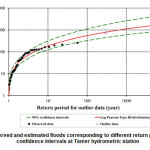
With regard to the lack of historical data in the study area, sensitivity analysis was used to assign a return period to the observed outlier. For this purpose, flood frequency analysis was performed using HEC-SSP 2.0 software considering different return periods for outliers. Sensitivity analysis results and estimated flow rates for different return periods are presented in Table 3. According to the above table, when a return period of 200 years and over is applied to outlier data, flood values do not change significantly for those return periods. Therefore, it can be concluded that frequency analysis results show less sensitivity to return periods of above 200 years. As a result, the return period of outlier (with flood magnitude of 783 m³/s) can be considered as 200 years. Figure 4 shows changes in design flood with 1000 and 10000 return periods when different return periods are assigned to outlier data. Figure 5 shows observed and estimated flow rates for different return periods with 95% confidence intervals at Tamer hydrometric station using an integration of outliers and systematic data.

Conclusions

In this study, the effect of outliers on flood frequency analysis was investigated using two analysis methods, one with complete series and the other by removing outlier data. The results indicated that although removing outlier data did not affect the determination of selected probability distribution (LP-III distribution), but removing outlier data reduced flood flow magnitude by 60% percent for 10000-year return period; from 3320 m³/s to 1340 m³/s. In integrating outlier data with systematic data, the method proposed by Water Resources Committee of the United States as well as HEC-SSP 2.0 software were used. In this method, the flood was estimated as 1907 m³/s for 10000 years return period by applying 200 years return period to outliers as well as correcting the distribution parameters of LP-III. Then, this value was reduced by 43% compared to the case the observed outlier was given the same value as other floods.
 

References
 

1. Adeyemo J., Olofintoye O., Optimized Fourier Approximation Models for Estimating Monthly Streamflow in the Vanderkloof Dam, South Africa, In EVOLVE - A Bridge between Probability, Set Oriented Numerics, and Evolutionary Computation. 288: 293-306 (2014).
2. Bouvard M., Design Flood and Operational Flood Control, General Report of the Question. 63:166 (1988).
3. England J., Jarrett R., Salas J., Data-based comparisons of moments estimators using historical and paleoflood data, Journal of Hydrology. 278:172-96 (2003).
4. Garcia F., Tests to identify outliers in data series. Pontifical Catholic University of Rio de Janeiro, Industrial Engineering Department, Rio de Janeiro, Brazil ( 2012).
5. Griffis, V.W., Stedinger J.R., 2007. Evolution of flood frequency analysis with Bulletin 17, Journal of Hydrologic Engineering. 12 (3):283-297 (2007).
6. Hagen V., Re-evaluation of design floods and dam safety. Proceedings, (1982).
7. Hamed K, Rao AR., Flood frequency analysis, CRC press (1999).
8. Heidarpour B., Panjalizadeh B., Ekramirad A., Hosseinnezhad A., Detection of Outlier in Flood Observations (A Case Study of Tamer Watershed), Journal of Research Jourrnal of Recent Sciences 4(3) (2015) (Accepted).
9. Hemmadi K., Akhood-Ali AM., Behnia AK., Arab DR., The Role of Updating Statistical Series in Assessment of Design Flood, a case study of Jareh Storage Dam, Iran-Watershed Management Science & Engineering. 1(2) (2007).
10. Hosking JRM., Wallis JR., Some statistics useful in regional frequency analysis, Water Resources Research. 29:271-81 (1983).
11. , Guidelines for determining flood flow frequency, Bulletin 17B, U.S. Geological Survey, Office of Water Data Coordination, Reston, VA. (1982).
12. , Cost of Temporary and Permanent Flood Control in Dams, Indian Committee on Large Dams, Central Board of Irrigation and Power (1997).
13. Kite GW., Frequency and risk analyses in hydrology, Fort Collins, Colo, Water Resources Publications.224 (1977.)
14. Pilon P., Harvey K., Consolidated frequency analysis (CFA), version 3.1. reference manual. Environment Canada, Ottawa (1994).
15. Singh, V., Entropy-based parameter estimation in hydrology. Vol. 30: Springer (1998).
16. Transportation A., Guidelines on extreme flood analysis, Civil Projects Branch, Edmonton, Alta (2004).
17. USACE., HEC-SSP Version 2.0, Statistical Software Package. Institute For Water Resources, Hydrologic Engineering Center (2010).