Estimation of Carbon Dioxide from Transportation Sector Based on Urban Data Availability
Abdu Fadli Assomadi 1
*
 , Rachmat Boedisantoso 1
, Agus Slamet 1
, Arie Dipareza Syafei 1
and Joni Hermana 1
, Rachmat Boedisantoso 1
, Agus Slamet 1
, Arie Dipareza Syafei 1
and Joni Hermana 1
1
Laboratory of Air Pollution Control and Climate Change, Department of Environmental Engineering,
Institut Teknologi Sepuluh Nopember (ITS),
Surabaya,
6011
Indonesia
http://dx.doi.org/10.12944/CWE.14.3.09
Copy the following to cite this article:
Assomadi A. F, Boedisantoso R, Slamet A, Syafei A. D, Hermana J. Estimation of Carbon Dioxide from Transportation Sector Based on Urban Data Availability. Curr World Environ 2019; 14(3). DOI:http://dx.doi.org/10.12944/CWE.14.3.09
Copy the following to cite this URL:
Assomadi A. F, Boedisantoso R, Slamet A, Syafei A. D, Hermana J. Estimation of Carbon Dioxide from Transportation Sector Based on Urban Data Availability. Curr World Environ 2019; 14(3). Available from: https://bit.ly/36l9AVD
Download article (pdf)
Citation Manager
Publish History

Introduction
Carbon footprint (CF) is a measure of human activities influence on the environment and climate change, and it is divided into two categories, i.e (1) the primary footprint, a measure of direct CO2 emissions from fossil fuels burning, such as from vehicles and transportation, and (2) the secondary footprint, a measure of indirect CO2 emissions, obtained from the life cycle of the products used in life. Both are a measure of energy consumption in a single or collection of activities. Unfortunately, the growth of CO2 emission has done enormous for developed and developing country, in the case for meet their population energy needed.1 The growth of CO2 emission has been a most challenging issues for developing country,2 like Indonesia.
In Indonesia, based on oil and gas statistic 2016, energy (fuel) consumption 72.3 – 66.9 million KL (kilo litre) and 96% is used by households, industry, and transportation.3 Transportation sector, in various studies and surveys, is a very large energy consumer and at the same a large carbon emitter. Generally, the quality and quantity of the transportation sector is identical to the condition of the road infrastructure available in the region.4
Road is a transportation infrastructure which includes all parts of roads, buildings and equipment that are intended for traffic, which is at ground level, above ground, below ground and/or water, as well as on the surface of the water, except railroad railway, highway and street wires.5 The road classification by function is (1) arterial road, is public road transport that serves the main freight function with the high travel distance and average speed characteristic, the number of driveways constrained efficiently; (2) collector road, is public road transport to serve the collector or divider with the medium travel distance and average speed characteristics (The number of driveways being restricted); and (3) local road, is public road to serve the local transport for short trips with low average speed characteristics and the number of driveways are not restricted.
The transportation sector contributes 23% of the emissions of total global CO2 emissions. Overall contribution of these emissions, 75% by road transport.6 This CO2 emissions problem should be handled optimally. One way of the handling is the emissions inventory and estimation in each region, to support the mapping and management of national emissions programs.
Various estimation methods have been published both nationally and internationally, and scientifically can be used to calculate the carbon emissions from a variety human activities, including transportation. World conventions provide guidelines according to the calculation method of the IPCC7 that can be used to calculate the carbon emissions for region or a city. The data required as inputs for the emission calculations, especially the quantity of fuels or energy, raw materials, or the nature of activity data units according to the needs of the IPCC method.8 Inappropriately, that required data however not available in the smallest urban areas of developing countries. It the fact, for most district and regency in developing country are very difficult to obtain the IPCC calculation. These countries do not have complete data in accordance with the IPCC required. For instance, the data transport sector in small towns in Indonesia, does not directly describe the quantity and the efficiency of fuel used, as the basis for calculating of emissions according to the IPCC. The available data that is considered to be valid enough, usually only the class and length of roads, number and type of vehicles, and the density or road loads. In other side, every country must report their carbon emission well every year. Thus the research effort was aimed to make the equivalent conversion of these data into equivalent carbon emission with fuel use and efficiency according to the IPCC.
Methodology
Review of Estimation Methods
There are many emissions models from transportation activities that have been developed and used. Some model in general is an estimation of CO2 emission based on fuel consumption or based on total km travelled.9 In others, model based on emission factors. Several studies are developed in international institutes or organizations, no literatures are fully cover the topics.10 The models used in this paper are classified into three equation principles since other known methods are identical and have the same principle with any of these three methods. The equations include:
The calculation that is based on the quantity of fuels, for example is in a mobile combustion model, it is the air modelling with mathematical calculations to predict the emissions of carbon dioxide (CO2). The calculation of CO2 emissions uses the amount of fuels consumed multiplied by the emission factor of the fuel type.11 The general equations used are:
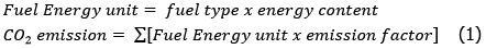
In mobile combustion equations, there are several data input, i.e.: 1) the amount of fuels that is derived from the overall amount of consumed fuels in the city, and 2) the CO2 emission factor for each type of fuel (in kg / TJ, obtained from the 2006 IPCC Guidance).
The calculation that is based on the quantity and type of contributors, is the air modelling with a mathematical calculation to predict the emissions of carbon dioxide (CO2). Some of models based travel forecasting and transportation analysis.12 Other model based on the type of vehicles that are grouped according to the type of its fuels, respectively. Equations used include:
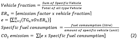
In these equations, there are several data inputs:
- Fraction of vehicles, obtained from dividing the number of each type of vehicles by the total number of all type vehicles, grouped as its fuel types.
- the gram per start emission rate for the specified technology group and pollutant = ER
- The number of vehicle trip origins = O
- The total number of vehicles grouped based on its fuel type consumptions = TG.
- Average fuel consumptions for each vehicle is obtained from the total of each type of fuel (petrol and diesel) in a region divided by the total number of vehicles that are grouped for each type of fuel consumption.
The calculation based on the methodology of IPCC (2006). This method is used for the development of national emissions report by countries, reported to the United Nations Framework Convention on Climate Change (UNFCCC). This method provides three-TIER approaches to meet the required degree of accuracy in accordance with the specifications of the data availability. The higher TIER gives better accuracy, but requires more complex of data and procedures. In principle, the best CO2 emissions calculation is based on carbon contents, amounts and types of fuel consumptions.8
Tier 1 methodology
Tier 1 approach is a simple method to calculate CO2 emissions, by multiplying the consumed fuels estimation by the general emission factor (default). The general equation of Tier 1 for transportation is:

Where the CO2 emissions in kg, with subscript a = types of fuel (diesel, premium, LPG​​, etc.), fuel estimated in tons and EF = emission factor (kg/ton).
Tier 2 methodology
This approach is similar to the Tier 1, with the emission factor is specific carbon contents for each country used for transportation. This approach depends on the category of fuel used by different vehicles and emissions standards. Equation 8 in Tier 1 can applied for Tier 2, but the emission factors must be calculated based on the actual fuel carbon content.
Tier 3 methodology
Tier 3 is more detailed than the Tier 2. This approach is based on activity data and emission factors with greater aggregates, but the results are more accurate than the Tier 1 and Tier 2, although it is more complex and difficult. However, the calculation of CO2 emissions using the IPCC Guidelines is recommended only using Tier 1 and Tier 2.8
Data Provided and Calculation Methods
The CO2 emission estimations must include all transportation activity in boundary of city reference.13 In this case, IPCC method strictly used, so it’s necessary to choose a city that has complete data as needed. For simulation, the chosen city is Surabaya, which has completely data of traffic, fuel consumption, vehicle types, class and length of road. Calculation of CO2 emission is completely carried out in several districts as reference and then specified by length or class of the road. The result of this calculation is a specific emission factor (SEF) that can be used for estimation of CO2 emission in another (general) district with limitation data of type and number of vehicles or length and class of roads, only.
All of data in this research provided by Surabaya City Government for 3 years. These data are class of road and length, traffic density for each class road, types of vehicles, and fuel consumption for all district. Calculation process generally schemed and provided in Fig. 1 for reference district and Fig. 2 for general district.
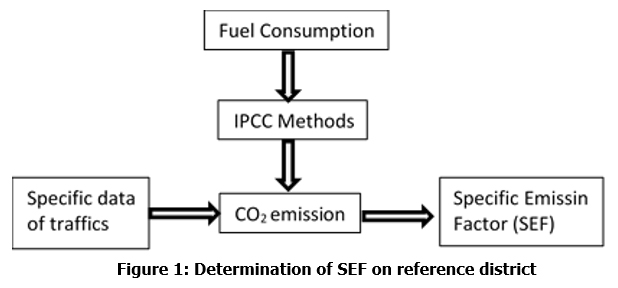 |
Figure 1: Determination of SEF on reference district Click here to view Figure |
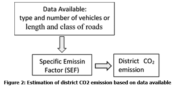 |
Figure 2: Estimation of district CO2 emission based on data available Click here to view Figure |
Result and Discussion
Inventory Data on Transport Sector
The construction of alternative methods for calculating carbon emissions in this paper are based on the principles of the 2006 IPCC formulation that used data inventory results from the transportation sector. The inventory was conducted through collecting primary data, survey data and observations, and the secondary data from relevant agencies. The main results of the inventory are:
- Data of the length of roads for each road class in the study area.
- Data of the road density and types of vehicles of each road class.
These data are generally available in most small towns or villages up to the district level in developing countries. While the data and the type of fuel consumption for transportation, as required by the IPCC to calculate carbon emissions, often are not well recorded until the level of small towns.
The Table 1 presents the inventory results of the length and the class roads in the study area (Surabaya city, East Java, Indonesia) in year condition of 2015. The entire study area was consisted of 5 locations and then subdivided into 30 study areas (district) as shown in Table 1. The distribution of the study areas based on the representative populations that are sufficient for the alternative models generated in this study.
Further, the calculation of potential CO2 emissions was approximated by predicting emissions for each road class. The calculation was based on the load or density for each road class in each study area. Thus, data that describes the load of each road class are of importance and it is presented in Table 2. The vehicles density of each road class was only counted for the groups of vehicles that are generally operated within the whole study area, i.e. motorcycles, passenger cars, mini buses, trucks and large buses.
Table 1: The area and length of each segment of the road class in the study area (km)
|
Location |
Number of Study Area |
AP (km) |
AS (km) |
CP (km) |
CS (km) |
L (km) |
|
Center zone |
4 |
6.32 |
16.98 |
0 |
44.39 |
107.85 |
|
Northern zone |
5 |
10.84 |
14.16 |
0.68 |
32.81 |
216.66 |
|
Eastern zone |
7 |
4.49 |
48.10 |
9.38 |
132.05 |
520.99 |
|
Southern zone |
8 |
9.54 |
15.35 |
17.10 |
84.26 |
631.65 |
|
Western zone |
6 |
1.89 |
11.39 |
5.67 |
48.59 |
352.84 |
|
Total |
30 |
33.08 |
105.98 |
32.83 |
342.10 |
1829.99 |
Notes: AP = primary arterial road; AS = secondary arterial road; CP = primary collector road; CS = secondary collector road; L = local road
Table 2: Average vehicle density (vehicles/hour) for each class of road
|
No. |
Vehicles Type |
AP |
AS |
CP |
CS |
L |
|
1. |
Motorcycles |
6795 |
4884 |
3313 |
4885 |
1200 |
|
2. |
Passenger cars (premium) |
1342 |
917 |
897 |
968 |
147 |
|
3. |
Passenger cars (diesel) |
727 |
265 |
241 |
323 |
52 |
|
4. |
Bus/mini trucks |
129 |
23 |
14 |
24 |
5 |
|
5. |
Trucks |
121 |
76 |
26 |
0 |
0 |
|
6. |
Large buses |
26 |
2 |
3 |
0 |
0 |
|
Total |
9141 |
6166 |
4495 |
6210 |
1404 |
|
Emission Factors and Emissions Calculation from Transportation Sectors
In principle, the carbon emissions is determined by two things: the amount of activity or loadings, and the emissions factors according to the type of activity or operational loads. The amount of activity or loading is obtained from the data processing of primary or secondary inventory results. While the emission factor, especially from the transportation sectors can be approximated by several methods. This emission factor is the average specific emission contribution from activities or loading of the source. Thus, the emission factor could be calculated based on each vehicle (according to its types), or per fuel consumptions, or per types of road considering its density/loads, and so on.
The IPCC 2006 formulation for estimating carbon emissions potential, in general, uses the activities of fuel consumption with emission factors for each fuel type consumed. The application of the IPCC formula will be a problem for the area that does not have a data record of fuel consumption, as in many areas of the developing world. Thus, determining the specific emission factor (SEF) on the basis of other activities will provide an alternative method for predicting carbon emissions in areas where the data availability is minimal. In this study, the SEF is expressed in two alternatives: 1) SEF based on data of the number and the types of vehicles 2) SEF based on data of the length and road class.
Table 3: Number of average emissions for each road class
|
Vehicle Types |
Average Emission (kgCO2/km.hour) |
||||
|
AP |
AS |
CP |
CS |
L |
|
|
Motorcyles |
468.8559 |
337.0057 |
228.6292 |
337.0563 |
82.7768 |
|
Passenger cars (premium) |
410.6287 |
280.6166 |
274.5141 |
296.2123 |
44.8343 |
|
Passenger cars (diesel) |
241.4406 |
87.9038 |
79.9724 |
107.3278 |
17.2418 |
|
Bus/mini trucks |
40.2163 |
7.1822 |
4.4753 |
7.3762 |
1.6001 |
|
Trucks |
56.0618 |
34.9662 |
12.0284 |
0 |
0 |
|
Large buses |
12.9210 |
0.8943 |
1.3894 |
0 |
0 |
|
Total |
1230.1243 |
748.5688 |
601.0088 |
747.9726 |
146.4530 |
Based on the results of traffic counting, as shown in Table 2, and the calculation using IPCC formulas, yielded the average carbon emissions per class road and for each vehicle type. The calculation results of the carbon emissions average for each road class as shown in Table 3. The data was subsequently used to determine the value of the two alternatives SEF based on the inventory data, i.e.:
- The SEF for each vehicle types, obtained by dividing the value of the emissions average for each road class with the each type and vehicles density of class road.

- The SEF for each road class, derived from the sum of carbon emissions average of all contributors types of vehicles on each road class.

The results of both SEF calculations are summarized in Table 4. Then the SEF data values are used to calculate the estimation of carbon emissions from transportation activities, based on the data availability in an area. If there is a region having a data for each class of road traffic counting, the SEF per vehicle will result in better calculation results. But if the region has only existing data of road class, the carbon emission calculation can be approximated by the SEF per class road. The use of the later emission factor still requires a region constant as a weighting factor that distinguishes one region to another based on the pattern of transportation.
Table 4: SEF alternative values ​​based on its data availability
|
Based on Fuel type, IPCC 2006 |
Alternative 1 |
Alternative 2 |
||||
|
Fuel Types |
SEF (kgCO2/l) |
Vehicle Types |
Specific Energy Consumption (l/vehicle.100km) |
SEF (kgCO2/ |
Road Class |
SEF |
|
Premium |
2,597.86 |
Motorcycles |
2.66 |
0.069 |
Primary Artery |
1230 |
|
Cars (Premium) |
11.79 |
0.306 |
Secondary Artery |
749 |
||
|
Diesel |
2,924.90 |
Cars (Diesel) |
11.36 |
0.332 |
Primary Collector |
601 |
|
Bus/mini trucks |
10.64 |
0.311 |
Secondary Collector |
748 |
||
|
Trucks |
15.82 |
0.463 |
Local |
146 |
||
|
Large buses |
16.89 |
0.494 |
||||
|
IPCC |
BPPT in Jinca et al., (2009) and Yamin et al., (2009) |
Calculation |
|
Calculation |
||
Verification of the emissions estimation based on the IPCC and both alternative methods
The next stage of this research was to perform emission calculations in study areas such as described in Table 1. The emission calculations used 3 methods: IPCC, alternative 1 and alternative 2.
Table 5: Carbon emissions estimation results by three alternative methods
|
Area |
Emission Estimation (ton CO2/years) |
Area |
Emission Estimation (ton CO2/years) |
Area |
Emission Estimation (ton CO2/years) |
||||||
|
IPCC |
Alt. 1 |
Alt. 2 |
IPCC |
Alt. 1 |
Alt.2 |
IPCC |
Alt. 1 |
Alt. 2 |
|||
|
1 |
44.2 |
48.7 |
51.4 |
11 |
49.4 |
63.2 |
57.0 |
21 |
51.4 |
59.6 |
59.6 |
|
2 |
80.7 |
86.3 |
91.4 |
12 |
105.8 |
118.0 |
121.4 |
22 |
51.8 |
56.5 |
59.4 |
|
3 |
93.3 |
94.5 |
99.0 |
13 |
178.8 |
195.0 |
205.0 |
23 |
49.3 |
53.9 |
56.8 |
|
4 |
107.6 |
114.9 |
121.4 |
14 |
208.5 |
224.8 |
245.8 |
24 |
141.3 |
159.5 |
162.3 |
|
5 |
84.0 |
101.6 |
97.8 |
15 |
109.6 |
131.8 |
129.5 |
25 |
127.9 |
137.9 |
146.0 |
|
6 |
69.9 |
82.3 |
80.5 |
16 |
83.4 |
95.2 |
97.6 |
26 |
151.7 |
164.2 |
173.7 |
|
7 |
85.9 |
91.6 |
96.5 |
17 |
161.4 |
174.9 |
185.0 |
27 |
51.9 |
63.3 |
59.9 |
|
8 |
52.0 |
60.9 |
57.1 |
18 |
170.3 |
188.0 |
198.7 |
28 |
95.1 |
101.6 |
104.1 |
|
9 |
108.1 |
112.8 |
118.7 |
19 |
103.8 |
114.9 |
120.8 |
29 |
105.5 |
118.5 |
119.0 |
|
10 |
83.3 |
98.7 |
97.7 |
20 |
75.4 |
85.1 |
89.5 |
30 |
164.5 |
170.6 |
186.3 |
It is intended to verify the results of the two alternative calculations by the IPCC as a reference. This verification is needed to compare the proximity of both alternative calculation methods with the reference (IPCC). The results of the calculation using the three methods are listed in Table 5, and the proximity of its value is shown in Fig.3.
 |
Figure 3: Value of carbon emissions from the three estimation methods Click here to view Figure |
Fig. 3 shows that the emission values generated by the two alternative methods tend to result in higher emission values as compared to the IPCC emission values. However, these values tend to be consistently and fairly close together. To investigate further the results of these two methods, both method values are correlated with the IPCC as shown in Fig. 4 and Fig. 5.
 |
Figure 4: Correlation of the alternative 1 emission calculation results to IPCC estimates Click here to view Figure |
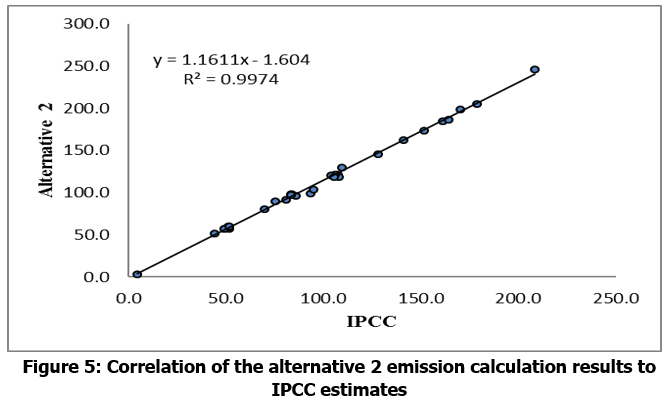 |
Figure 5: Correlation of the alternative 2 emission calculation results to IPCC estimates Click here to view Figure |
Fig. 4 shows the correlation values between by the alternative 1 data with the data calculated by the IPCC. It appears that both values have the same tendency or linear correlation. The value of correlation (R2) for the alternative 1 and the IPCC was 0.990. While the correlation factor for the alternative 2 with the IPCC values are shown in Figure 3. The R2 values for the alternative 2 and the IPCC was 0.997. Hence, the alternative 2 has a linear correlation value better than the alternative 1. However, both these alternatives provide excellent values and close to the value given by the IPCC. Both of correlation values indicated the priority use for the availability of data.
The calculation of standard errors for the two alternative data correlation with the IPCC gives the following results:
- Alternative 1 provides the results of 112.3 + 4.7 ton CO2/years
- Alternative 1 provides the results of 116.3 + 2.8 ton CO2/years
Thus, both alternative methods of this research can be used to calculate estimates for the carbon emissions from the transportation sector according data availability. If there are sufficient data for all three methods, the priority calculation could use the IPCC method, then the alternative 2 which is based on the number and type of vehicles in operation, and the latter using an alternative 1 which is based on the length and class of roads.
Conclusions
Two alternative methods for calculating carbon emissions of the transportation sector can be applied. The alternative 1, the SEF in kg CO2/vehicle.km, based on the type and number of vehicles in operation; Alternative 2, the SEF in kg CO2/hr.km, based on the length and class of roads. Both of these alternatives provide a good correlation with the results of the IPCC. Both can be used independently in accordance with the availability of existing data in the regions. Alternative 2 provides results that are closer to the IPCC by the correlation value 0.997 with the standard error of 2.8 ton CO2/years, as compared to the alternative 1 (the correlation value of 0.990 and a standard error of 4.7 ton CO2/years).
Acknowledgement
This study goes on support of Ministry of National Education and Higher Education, 2015, Surabaya City Government, 2015, and Research and Community Service Institutions of ITS. All of secondary data is provided by Environmental Agency of Surabaya City Government, accessed in 2015.
References
- Modi A, Bhojak N. P. Study the Carbon Emission Around the Globe with Special Reference to India. Current World Environ. 2013;8(3) 429 – 433.
CrossRef - Akhtar S, Sahibzada N. I, Saif S, Inayat S, Ahmad S. R. Carbon Footprint of a Beverage Bottling Plant in Lahore, Pakistan. Current World Environ. 2017;12(2) 222 – 230.
CrossRef - Directorate General of Oil And Gas. Oil and Gas Statistic 2016. Ministry of Energy and Mineral Resources, 2016; 50 – 51.
- Indonesia Ministry of Environment. Report, Indonesian Environmental Status year 2007, KLH-Jakarta. 2008;XXV
- Act of the Republic Indonesia No 38 year 2004 about Road. President of Indonesia. 2004
- Regmi, M. B., & Hanaoka, S. A Framework to Evaluate Carbon Emissions from Freight Transport and Policies to Reduce CO2 Emissions through Mode Shift in Asia. Tokyo 152-8550, Japan: Department of International Development Engineering, Graduate School of Science and Engineering, Tokyo Institute of Technology. 2011.
- Eggleston S. L. IPCC guidelines for national greenhouse gas. Hayama, Japan: Institute for Global Environmental Strategies. 2006.
- IPCC. Guidelines for National Greenhouse Gas Inventories. Geneva: IPCC. 2006.
- Angelakogluo K, Gaidajis G, Lymperopoulos K, Botsaris P. N. Carbon Footprint Analysis of Municipalities – Evidence from Greece. Journal of Engineering Science and Technology Review. 2015;8(4) 15 – 23.
CrossRef - Radu A. L, Scrieciu M. A, Caracota D. M. Carbon Footprint Analysis: Toward a Project Evaluation Model for Promoting Sustainable Development. Int. Economic Conf. of Sibiu 2013. Elsevier, Procedia Economics and Finance. 2013; 6 353 – 363.
CrossRef - Dunlap R. A. A Simple and Objective Carbon Footprint Analysis for Alternative Transportation Technologies. Energy and Environment Research. 2013; 3(1) 33 – 39.
CrossRef - Armstrong J. M. and Khan A.M. Modelling Urban Transportation Emission: Role of GIS. Elsevier Journal of Computer, Environment, and Urban System. 2004; 28(4) 421 – 433.
CrossRef - Assomadi A.F, Widodo B, Hermana J. The Kinetic Approach of NOx Photoreaction Related to Ground Measurement of Solar Radiation in Estimates of Surface Ozone Concentration. International Journal of ChemTech Research. 2016; 9(7)182 – 190.


