Evaluation of the Drought Trend Alongside of Change Point: A Study of the Purulia District in West Bengal, India
Shrinwantu Raha
*
 and Sayan Deb
1
Department of Geography,
Bhairab Ganguly College,
Belgharia,
West Bengal
India
http://dx.doi.org/10.12944/CWE.18.2.10
Copy the following to cite this article:
Raha S, Deb S. Evaluation of the Drought Trend Alongside of Change Point: A Study of the Purulia District in West Bengal, India. Curr World Environ 2023;18(2). DOI:http://dx.doi.org/10.12944/CWE.18.2.10
Copy the following to cite this URL:
Raha S, Deb S. Evaluation of the Drought Trend Alongside of Change Point: A Study of the Purulia District in West Bengal, India. Curr World Environ 2023;18(2).
Download article (pdf)
Citation Manager
Publish History

Introduction
Drought is a recurring, naturally occurring climatic phenomenon that cannot be avoided1,2. The nature and intensity of droughts are related to the lack of precipitation, which further leads to the decreasing trends in the soil moisture1-4. Droughts occur in almost all climatic regions with varying intensities and trends 5. Over 4 types of droughts, meteorological drought is the most common and complex in nature6,7. In recent times, researchers from all over the world are more concerned about the spatio-temporal assessment of meteorological drought. For example, Spinoni et al.8 analysed the drought database (from 1951 to 2016) in three spatial scales (i.e., global, macro-regional, and country scale). Abbasian et al.9 evaluated the drought on the Lake Urmia Basin by introducing a new precipitation-temperature deciles index. Pandey et al.10 estimated the drought of Central India using the TRMM version 7 (TRMM-3B43 V7) precipitation data from 1981 to 2016. They found that the drought was shifting from the West towards the East. Datta et al.11 estimated meteorological drought during 1960-2013 over the Ghatprabha river basin and found its' increasing trend between 2005 to 2013. Bisht et al.12 evaluated the drought of India using 9 projected global circulation models and found the severity of the droughts in the eastern sections of India. Kar et al.13 measured the drought of West Bengal at several time steps and found its' extremity in Western portions of the West Bengal, especially over the Purulia. Kundu and Mondal14 analyzed the trends of the precipitation time series during 1901-2002 over West Bengal and found its' decreasing nature over Purulia. They had further concluded the necessity of assessment of drought on this tract. Considering such contexts, assessment of the drought trends over the Purulia is a noble attempt.
There are different meteorological drought indices such as; Rainfall Anomaly Index (RAI), Effective Drought Index (EDI), China Z Index (CZI), and Standardized Precipitation Evapotranspiration Index (SPEI)). Standardized Precipitation Index (SPI) is considered in this research because of its' flexibility and adaptability at different climatic regions15-18. Also, the fundamental advantage of SPI is its’ capability of monitoring both dry as well as the wet periods in long- and short-term time scales and duration19. Therefore, considering those flexibilities of SPI and following the recommendation of World Meteorological Organisation20, this research has utilized the SPI to detect drought at yearly and seasonal scales.
Similar to this, a number of parametric and non-parametric tests have been extensively utilised globally to identify trends, their amplitude, and their change point in both meteorological and hydrological time series. Non-parametric tests yield better results than the parametric method, when the meteorological variables are skewed from the normal distribution21. Mahajan and Dodamani22 estimated the tendency (trend) of drought over the Krishna basin at southern Maharastra using the Mann-Kendal trend and Sen’s slope. They found the monsoon phase with a positive trend (2 significant positive trends), while the pre-monsoon time scale was noted with a negative trend (at 41 stations). During the post-monsoon season, no significant trend was detected. Sharma and Goyal23 estimated the drought trends of India for the last decade (1901 to 2002) using the Sen's slope value. They found eastern and north-eastern portions with an upward trend and southern regions with decreasing trends. Vishwakarma et al.24 discussed droughts (during 1988-2018) of Sagar, division of Madhya Pradesh using the Mann Kendal test. A significant positive trend was marked by them in Pre-monsoon (PM) and Post-monsoon seasons (PMW). Bhunia et al.25 discovered the change point in the time scales of precipitation (in the Purulia) and found its’ shifting nature during 1990s. Further, they stressed over the micro-level assessment of the drought phenomena to understand the local level climatic features meticulously. Das et al.26 analyzed drought during the Indian summer-monsoon period using Mann Kendall test (MK) and Sen's slope. They discovered a positive trend of drought in India's eastern regions and a major decreasing drought trend along the West Coast and in western India during rainy (monsoon) season, Using the grid level daily precipitation data over India from June to September, Kumar et al.27 projected dryness for the years of 1951 to 2007. They discovered a low drought in the western portions of India and a moderate drought in the eastern sections of India.
Therefore, it will be very beneficial to investigate the drought trend in India at the sub-regional and local levels, which was not done in prior research. Agriculture is a major economic activity in both West Bengal and India. Despite the recent progress of industrialization in Purulia, the fundamental pillar of the economy depends on the gross production of agricultural commodities28. As a predominant drought-prone district, the micro-level assessment of drought is desperately needed for the Purulia for efficient agrarian planning. As previous studies were not focused on assessing the drought trend in this district, the aim of the research is to analyse and estimate the trend of the drought along with the change point using the Standardized Precipitation Index (SPI), Mann-Kendall test (MK), and Sen's slope.
Study area
The Purulia, an extended section of the Deccan Trap, is located in the western tracts of West Bengal. The districts of Bankura and Paschim Medinipur form its’ eastern border. Bardhaman district in West Bengal and Dhanbad district in Jharkhand state form its’ northern and western borders, respectively. Bokaro and Ranchi district in Jharkhand state form its’ western and southern borders. The total area of the region is 6250 Square Km. Several rivers traverse the district of Purulia. The most significant ones are Kangsabati, Kumari, Silabati (silai), Dwarakeswar, Subarnarekha, and Damodar. Despite the district's many rivers, the terrain's undulations cause 50% of the water to run off. The Purulia has tropical Savanna climate. The region is having a substantial amount of its’ rainfall concentrated during the monsoon seasons (1100 to 1500mm precipitation)29. Extremely hot summers and chilly, low winter temperatures are experienced in the area. The region experience near about 52ºC temperature in the summer and a very cold 3.8ºC in the winter.The summer months are exceedingly dry. 50% of the water in the soil evaporates as runoff because of its’ poor ability to retain moisture30. The relative humidity is observed in the monsoon season is from 75% to 90%. According to SAFE31, Purulia was the exceptional hit of drought, and agricultural production fall to 27% from 2011 to 2016. In 2017, drought caused almost 280,000 hectares of agricultural land to be barren32. Generally, there exists a desiccating effect of drought on the normal cropping pattern or cropping system in the Purulia33,34. Drought in the early season generally results in 2 to 3 weeks delay in the agricultural crop production and aquaculture35, 36. Red and laterite soil with undulated land are available in the Purulia District, and this type of soil cannot store the water 37,38. As per the Census of India,39, the district's total population is 2930115, out of which 87.26% reside in the rural areas and 12.74% in the urban areas. Out of the total agricultural landholdings, approximately, 73% belong to the marginal farmers, who have several fragmented lands40,41. Only 15% of the net cropped area is under multi-crop cultivation, even though net cropped land accounts for 57% of total land42. Kharif paddy farming covers 83 percent of the total net-cropped area. The crops are primarily rainfed, and fertilizer consumption per unit area is often modest43. As a result, the production per hectare is comparatively low. The drought condition of 2010 ended their only means of livelihood44. Therefore, in order to deal with drought, the trend of meteorological drought along with the change point is absolutely necessary. The study area's location was shown on a map in Fig. 1.
Methodology and datasets
The whole methodology was implemented through a 5-step process in this research (Fig. 2). The methodology began with the gathering of information about the precipitation and concluded with the evaluation of drought during the both phases, which are the pre- and the post-change point. The process was explained (Step by step) as follows:
First step- Collection of the precipitation data
The station specific data for the precipitation time series (daily-basis) were collected from CFSR (“Climate Forecast System Reanalysis”), SWAT based web portal45. CFSR-SWAT is a validated and trusted database, which bears an open access licence for their users25,46-48. This portal stores the data from 1979 January to July 2014 on the daily basis. Those data were collected first and then formatted in a monthly time frame. Next, the monthly data was divided into 4 series i.e., 1) Annual or yearly series (A) 2) March to May- Pre-monsoon series (PM) 3) June to October- monsoon series (MS) 4) November to February- Post-monsoon with winter series (PMW). The mean and standard deviation of precipitation were demonstrated in the Table 1. Fig. 2 expressed the 8 meteorological stations within the study area.
Second Step-Determination of drought using Standardized Precipitation Index (SPI)
SPI is a popular flexible index to detect and characterize meteorological drought49,50. SPI was first constructed by McKee et al.51, and thereafter, it was further developed by Edwards and McKee52. They measured precipitation anomalies at a given location by comparing observed precipitation with the long-term historical precipitation for a specific period. The World Meteorological Organization (WMO) had recommended SPI for several meteorological and hydrological services20. In this research, the SPI was calculated in accordance to the guideline of World Meteorological Organization (WMO)20:
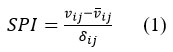
The total difference between the data points for the whole time series of precipitation, and the extended long-term precipitation means was calculated as the first step. The data points at each time frame (i.e., here j-th) were marked as vij, the average of the whole column of the precipitation was illustrated as and the Standard Deviation of the precipitation column was marked as the ; therefore, the process was initialised with the eq.(1)53
Thom54 discovered that the gamma Probability Distribution Function may be used to systematically match the time series of different climatological variables. The precipitation series was therefore fitted with the gamma Probability Distribution Function54 in the following step for the purpose of 1) transforming the precipitation value to the zero events, and 2) the adjustment of the standard deviation to 1.0. The Gamma Distribution Function was denoted as follows by Eq. (2):
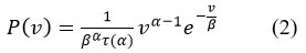
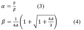
Where, is the Gamma Distribution Function, v is the amount of precipitation (v>0), is the shape parameter, the scale parameter is the (. Now shape and scale parameter and were determined as follows (Eq. 3 and Eq. 4):
Where, A was obtained using the following equation (Eq. 5 and Eq.6):
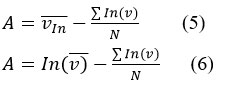
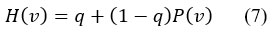
Here, the precipitation data was converted to lognormal values and the statistics A, and (shape and scale parameters) were computed. Here, all cases N is the number of observations. Now, since the gamma function is undefined for v = 0 and a precipitation distribution may contain zero. Then, the cumulative probability becomes (Eq. 7):
Where, q is the probability of zero events. In this research, the SPI was calculated by the MDM software, a free tool provided by the Agrimetsoft team54. The above procedures are merged into this software4.
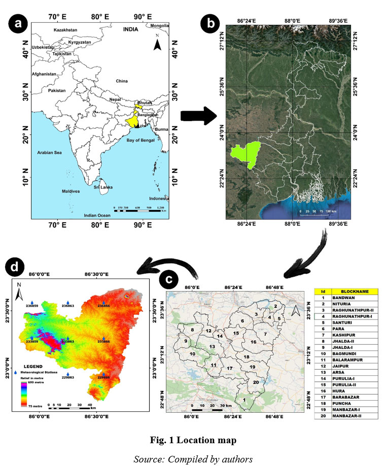 | Figure 1: Location map.
|
Source: Compiled by authors
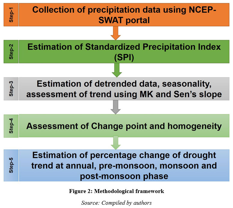 | Figure 2: Methodological framework.
|
Source: Compiled by authors
Third Step- Estimation of detrended data, assessment of trend and seasonality
Trend from the detrended data (TFPW series)
The basic assumption of the Mann-Kendal (MK) and as well as for the Sen's slope is that the data is randomly ordered, and no trend typically exists in the dataset. But the true nature of hydro-meteorological variables is that it bears a significant autocorrelation coefficient67. A straight-forward ‘Pre-Whitened’ procedure was framed by Von Storch68 but the method seems to be inappropriate for the negative auto-correlation69,70. Therefore a trend free two-tailed Pre-whitening method by Yue et al.71 was applied through the following steps:
Sen's slope estimator ? was computed from the SPI data using equation (18). Now, to retrieve the detrended series the eq. (8) and eq. (9) were utilised:
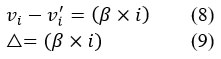
Where, ? is the Sen’s slope, is the i-th data of original precipitation time series. is the series of after initial removal of auto-correlation. is the difference between and .The lag-1 serial or autocorrelation coefficient was calculated for the new trend-free (detrended) series. Following the Tabari and Talaee72 methodology, if r1 significantly deviated from the value 0 the SPI dataset was considered the serially uncorrelated or independent dataset. Then the MK test method and Sen’s slope were directly applied to that dataset. If the above case did not occur, the dataset was regarded as the serially correlated dataset, and the trend test was applied in the following way (Eq. s10 ,11,12)
From Eq. (8) we get,
Where, ? is the Sen’s slope, v is the original precipitation time series. Eq. (12) is the final TFPW series on which further mathematical operations were implemented. The 'Trend-change'73 is a helpful R-package utilized to determine the TFPW series in this research.
Trend estimation using Mann-Kendall test (MK test)
There are many statistical methods for detecting trends, and each method has their advantages and disadvantages56. The Mann-Kendall statistical test is widely acknowledged as a non-parametric test to find the tendency (trend) of all meteorological variables57. Here, the MK trend test denotes the trend of meteorological drought based on the SPI. Mann Kendall (MK) test is a kind of statistical index, which is not affected by the extremity of the sample (data) points58. The Mann Kendall test (S)59-61 was recommended by the World Meteorological Organisation20, and this procedure was used here through the Eq. (13):
Where, S denotes the value of the MK test statistic; n is the total count of the whole data, indicates the value of j (j>i)-th data, and is the signum function in Eq. (14):

The positive S indicates the upward trend, and the negative value indicates its' reverse. The S is taken as the normally distributed, where N ? 8. The mean and the variance of S are computed as follows in the Eq. (15) and Eq. (16):
Where, the total count of ties among the groups is represented by , and is the total count of the whole data. When there are more than 30 samples, the standard normal format of was calculated as follows 62,63 in the Eq. (17):

Positive trends of Z value are marked with a positive trend, and negative Z value is marked a negative trend of drought. Trends were estimated at a specific ? significance level (here, ? is .05).
Sen's slope ()
The magnitude of trend denoted here as a Sen’s slope ( )in the given SPI time series was measured in the following way64,65 Eq. (18).
In the above equation (18), 1i is the i-th observation of the precipitation time series v and the j is the j-th observation of the time series of precipitation marked as v. According to Tabari et al.66, is the value of median noted with all of the possible paired combinations. Therefore, the extreme values are not included in this test.
Estimation of seasonality using Wavelet Transform (WT)
Wavelet transform is an advanced mathematical tool fitted for providing information of time-recurrence signal74. Grossmann and Morlet developed it in 198475. WT is widely used in time series forecasting and trend analysis of hydro-meteorological variables76. The Fourier transform (FT), segregates the signal into smooth curve (sinoids), which has an infinite duration, whereas the WT divides the signal into wavelets of the finite segments with zero mean1. These wavelets are localized both at frequency and time domains. The wavelet analysis was expressed here as follows77 (Eq. 19):

Where, is the Wavelet Transform Function; is the frequency, is the shifting phase with time t, is the conjugate of the original which is determined by the wavelet function generator. v(t) is the original time series of precipitation. In this study, the Morlet wavelet transform78 was used to determine the periodic structure of annual and monthly (seasonal) SPI time series. The wavelet series by Morlet consists of a plain wave, which was moduled by a Gaussian component79.The "angular frequency" v is considered as 3 to make the analytic curve by the Morlet Wavelet80,81.
Fourth Step-Assessment of the change point and homogeneity
Change point estimation using Pettitt Mann-Whitney U test
The Pettitt Mann-Whitney test was adopted to identify the best possible single change point within the SPI time series. The two samples for the SPI time series are the annual and monthly time steps: V1……...VTand Vt+1 …… Vt (Eq. 20):
The index is
.jpg)
for any t
Where, is a signum function that returns a real number.
Let, another index Ut be defined as (Eq. 21)
.jpg)
The most appropriate change point here denoted as t is defined as the phase K (in between upper bound and lower bound) where the Ut attains its’ maximum value (Eq. 22):

The likelihood (p) of a change point is being at the phase surrounding the particular point where the Ut is approximated by (Eq. 23)
Further it can be introduced, for l ? t ? T, as (Eq. 24)
Where, is the Dummy variable for the change or shift point. T is time. is the highest value at the time t.
And it is defined as, (Eq. 25).
Where, is the Pettitt Mann-Whitney test.
In this research, the region between the upper and lower bound of the Mann Whitney U statistic was considered the change point region80. Since the change point phase for monthly and annual scales varied between 1988 and 1989, the period was used as the change point phase.
Kruskal-Walis test (H) to analyse the homogeneity
To ascertain whether there is a most probable difference between two phases (before and after the shift point), the Kruskal-Walis Chi-square test was used. The procedure is as follows82:
Rank the observations from the smallest to largest and give them weightage accordingly
Then Chi-square test83 was applied
In case of no ties exist; the H was obtained as follows (Eq. 26)
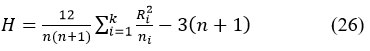
Where, H is the value of Kruskal-Wallis test, the i-th group, is the sum of all observations, and the sum of the ranks in the i-th group is denoted as .
If the number of identical observations exceeds 25% of the number of the samples, the H can be modified in the following way (Eq. 27):
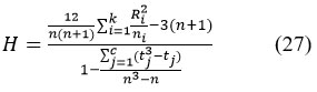
Here, is the total count of all the tied groups and is total dimensions of all j which is the tied group. When ? 5, the H accurately coincides with the ?2 distribution. If H coincides with the degrees of freedom denoted as ?2 (1-?, k-1) ,the hypothesis will be rejected72. In this study, a level of 95% was used.
Fifth Step-Estimation of percentage change of drought
Percentage change of trend in both the phases (i.e, before and after) was expressed as mentioned below84 (Eq. 28):
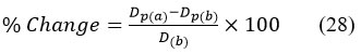
Where, is the MK or Sen’s slope value after the change point, and is the drought assessment factor before the shift; and the is the reference period, the drought evaluation parameter prior the shift of the change point.
To visualize all of the maps and diagrammes, Inverse Distance Weightage Method (IDW) was applied in ArcGIS 10.4.
Results
Descriptive statistics of annual and seasonal precipitation
The mean, SD, and CV of precipitation were portrayed in the Table 1. The stations with the largest and smallest mean annual precipitation were observed at stations 229866 (2nd station) and 236859, respectively. In the annual series, the highest standard deviation of precipitation was identified at station 229866 (2nd Station). On the other hand, the lowest standard deviation of precipitation was noticed at station 229863 (1st station) in the annual series (A). The lowest and largest coefficients of variation for precipitation were found at stations 229863 (1st station) and 233866 (5th station), with 18.25% and 312.39%, respectively.
Similarly, 229863 (1st station) and 229866 (2nd Station) stations, had the highest (2193.199 mm) and lowest (539.853 mm) mean and standard deviation of precipitation, during the pre-monsoon series (PM). At this phase, the lowest and highest precipitation variation were noticed at stations 233866 (5th station) and 236859. The lowest mean and standard deviation of precipitation were identified at the station 236859 during the monsoon (MS) season. On the other hand, the highest mean (13302.771mm.) and standard deviation (6487.936 mm.) of precipitation were observed in stations 233866 (5th station) and 229866 (2nd Station), respectively. Stations 236863 (7th station) and 229863 (1st Station) had the highest and lowest variability during the monsoon phase respectively. At the post-monsoon phase (PMW), the highest precipitation variability was observed at stations 233859 (3rd station), 236863 (7th station), and 236866 (8th station), with approximately 194% coefficient of variation. Station 229863 (1st Station) had the lowest variability of precipitation during this phase. The highest (16940.053mm.) and the lowest mean (407.334mm.) precipitation in the post-monsoon phase (PMW) were recorded at stations 2338632 and 229863 (1st Station), respectively.
Table 1: Descriptive statistics table denoted the annual, mean, SD and CV of the precipitation (1979-2014).
Station name | Longitude | Latitude | Season | Mean precipitation (mm.) | Standard Deviation (SD) | Coefficient of Variation (%) ( |
229863 (1st station) |
86.25
|
22.9487
| Annual (A) | 1808.272 | 330.059 | 18.252 |
Pre-Monsoon (PM) | 539.853 | 295.506 | 54.923 | |||
Monsoon (M) | 12093.408 | 5799.877 | 47.659 | |||
Post-Monsoon (PMW) | 407.334 | 120.085 | 29.480 | |||
229866 (2nd station) |
86.5625
|
22.9487
| Annual (A) | 2037.008 | 605.171 | 29.708 |
Pre-Monsoon (PM) | 2193.199 | 2558.716 | 116.665 | |||
Monsoon (M) | 13108.215 | 6487.936 | 49.495 | |||
Post-Monsoon (PMW) | 410.706 | 152.910 | 37.231 | |||
233859 (3rd station) |
85.9375
|
23.2609
| Annual (A) | 1717.043 | 404.121 | 23.530 |
Pre-Monsoon (PM) | 1678.181 | 2119.245 | 126.282 | |||
Monsoon (M) | 10302.90 | 5437.539 | 52.776 | |||
Post-Monsoon (PMW) | 15424.76 | 29942.4 | 194.118 | |||
233863 (4th station) |
86.25
|
23.261
| Annual (A) | 1835.864 | 575.07 | 31.324 |
Pre-Monsoon (PM) | 1888.980 | 2340.331 | 123.89 | |||
Monsoon (M) | 11381.822 | 6038.951 | 53.057 | |||
Post-Monsoon (PMW) | 16940.053 | 32982.56 | 194.701 | |||
233866 (5th station) |
86.5626 |
23.261 | Annual (A) | 2008.751 | 643.03 | 312.388 |
Pre-Monsoon (PM) | 660.691 | 346.821 | 52.49 | |||
Monsoon (M) | 13302.771 | 6241.709 | 46.920 | |||
Post-Monsoon (PMW) | 462.301 | 149.934 | 32.431 | |||
236859 (6th station) |
85.9375 |
23.573 | Annual (A) | 1294.573 | 434.157 | 33.536 |
Pre-Monsoon (PM) | 1395.762 | 1814.873 | 130.027 | |||
Monsoon (M) | 7898.823 | 4280.051 | 53.274 | |||
Post-Monsoon (PMW) | 12055.28 | 23252.99 | 192.886 | |||
236863 (7th station) |
86.25 |
23.573 | Annual (A) | 1427.940 | 500.381 | 35.042 |
Pre-Monsoon (PM) | 1542.809 | 1939.737 | 125.727 | |||
Monsoon (M) | 8756.843 | 4804.844 | 54.869 | |||
Post-Monsoon (PMW) | 13244.423 | 25643.65 | 193.618 | |||
236866 (8th station) |
86.5625 |
23.573 | Annual (A) | 1571.319 | 540.751 | 34.413 |
Pre-Monsoon (PM) | 1698.443 | 1982.884 | 116.747 | |||
Monsoon (M) | 10086.22 | 5505.104 | 54.580 | |||
Post-Monsoon (PMW) | 15105.66 | 29303.22 | 193.988 |
(Compiled by authors)
Estimation of periodicity of drought using Morlet Wavelet transforms
The periodic nature of drought at the annual (A) and seasonal scales were portrayed in the Fig. 3 using the Morlet Wavelet Transform. Here, time and periodicity were displayed on the x and y-axis respectively. High significance (10% significance level) against the joint periodicity scale was denoted by the white lines in Fig. 3. At the annual scale, drought ranged from 0.25 to 0.5 months from 1979 to 1988. From 1989 to 2003, the periodicity of drought fluctuated from 0.5 to 0.55 months. From 2006 to 2014, periodicity fluctuated from 0.27 to 0.51 months. 2004 to 2005 was noticed with an inconsistent periodicity. Except from 2004 to 2006, the total annual phase was identified with a higher concentration of power (Fig. 3a). In the pre-monsoon phase (PM), the drought was noticed with a significantly high concentration level from 1979 to 1988. But from 1989 to 2005, the drought was identified with a relatively low concentration of power. At this phase, inconsistent periodicity was observed after the year 2005. At the pre-monsoon phase (PM), drought varied with 0.00 to 16.32 wavelet power (Fig. 3b). At the monsoon phase (MS), periodicity of drought was noticed with significantly high-power levels during 1979 to 1993 and 2007 to 2010. From 1994 to 2006 and after 2010, the periodicity of the drought was inconsistent. Overall, the periodicity of drought at monsoon season (MS) varied from 0.00 to 18.30 wavelet power level (Fig. 3c). At the post-monsoon phase (PMW), a significant periodicity of droughts was observed from 1979 to 1985 and 1997 to 2000 with a higher concentration of power. Droughts were noticed from 2007 to 2014 with a significant periodicity with a low power concentration (Fig. 3d). 2001 to 2006 was detected with inconsistent periodicity at this phase.
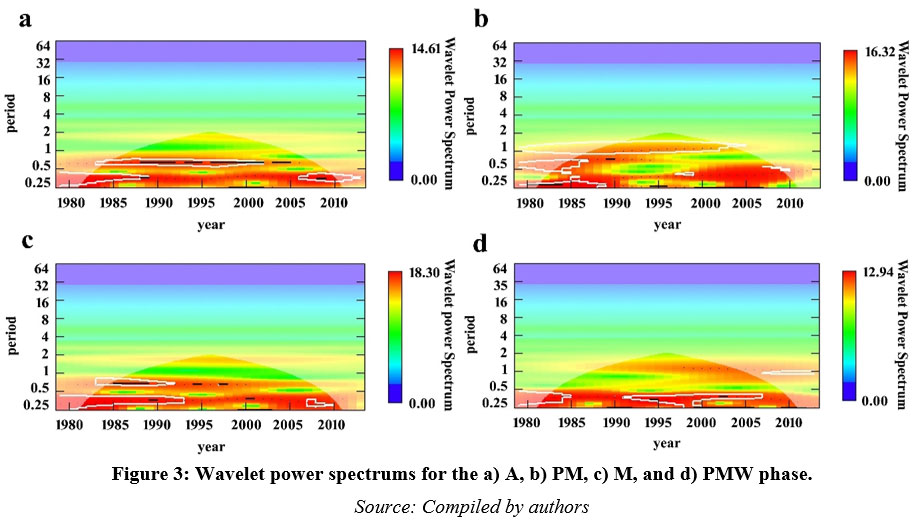 | Figure 3: Wavelet power spectrums for the a) A, b) PM, c) M, and d) PMW phase.
|
Source: Compiled by authors
Estimation of change point at annual and monthly series
The Pettitt Mann-Whitney test was applied for annual and monthly series to determine change points. Both for annual (A) and monthly series, 1988-1989 was obtained as the change point. Pre-monsoon (PM), monsoon (MS), and post-monsoon (PMW) phases were included in the monthly series. Thus, for both annual and monthly series, 1979–1987 represented the pre–change point phase, and 1990–2014 represented the post–change point phase (Table 2). The Kruskal-Wallis homogeneity test (KW) was used to examine the mean deviation before and after the change point in both annual and monthly time series (in this case, SPI series). By utilizing the KW test, the time series of the drought was heterogeneous at all stations at the annual series (Table 3). At pre-monsoon (PM) (Table 4) and post-monsoon phase (PMW) (Table 6), five stations were noticed with homogeneous nature, whereas other stations were detected with the reversed feature of the previous. At monsoon season (MS) (Table 5), five stations were seen with a heterogeneity.
Table 2: Pettitt-Mann Whitney test result for annual and monthly series (pre-monsoon, monsoon and post-monsoon series included)
Station name | Annual series (Change point) ** | Monthly series (Change point) ** | Change point taken (for both annual and monthly series) | Before change point series (for both annual and monthly series) | After change point series (for both annual and monthly series) |
229863 (1st Station) | 1988 | 1988 | 1988-1989 | 1979-1987 | 1990-2014 |
229866 (2nd Station) | 1989 | 1988 | 1979-1987 | 1990-2014 | |
233859 (3rd station) | 1988 | 1989 | 1979-1987 | 1990-2014 | |
233863 (4th station) | 1988 | 1989 | 1979-1987 | 1990-2014 | |
233866 (5th station) | 1989 | 1988 | 1979-1987 | 1990-2014 | |
236859 (6th station) | 1989 | 1988 | 1979-1987 | 1990-2014 | |
236863 (7th station) | 1988 | 1989 | 1979-1987 | 1990-2014 | |
236866 (8th station) | 1989 | 1989 | 1979-1987 | 1990-2014 |
** For monthly and annual series, the confidence interval or the upper and lower boundary limits are taken as the phase of the change point (Compiled by authors)
Table 3: Kruskal-Wallis (KW) homogeneity test for annual series (change point is 1988-1990).
Station Name | KW test (Chi-Square value) | Prob.>Chi-square | Series homogeneity |
229863 (1st Station) | 4.64 | 0.03 | S1 |
229866 (2nd Station) | 5.47 | 0.01 | S1 |
233859 (3rd station) | 4.50 | 0.03 | S1 |
233863 (4th station) | 5.59 | 0.01 | S1 |
233866 (5th station) | 5.83 | 0.01 | S1 |
236859 (6th station) | 4.27 | 0.03 | S1 |
236863 (7th station) | 5.79 | 0.01 | S1 |
236866 (8th station) | 6.44 | 0.01 | S1 |
S1- Heterogeneous group, S0- Homogeneous group (Compiled by authors)
Table 4: Kruskal-Wallis (KW) homogeneity test for pre-monsoon series (change point is 1988-1990).
Station Name | KW test (Chi-square value) | Prob.>Chi-square | Series homogeneity |
229863 (1st Station) | 0.36 | 0.54 | S0 |
229866 (2nd Station) | 7.80 | 0.03 | S1 |
233859 (3rd station) | 1.04 | 0.31 | S0 |
233863 (4th station) | 0.12 | 0.72 | S0 |
233866 (5th station) | 7.85 | 0.01 | S1 |
236859 (6th station) | 7.85 | 0.01 | S1 |
236863 (7th station) | 1.92 | 0.16 | S0 |
236866 (8th station) | 3.80 | 0.05 | S0 |
S1- Heterogeneous group, S0- Homogeneous group (Compiled by authors)
Table 5: Kruskal-Wallis (KW) homogeneity test for monsoon series (change point is 1988-1990).
Station Name | KW test (Chi-square value) | Prob.>Chi-square | Series homogeneity |
229863 (1st station) | 1.92 | 0.16 | S0 |
229866 (2nd Station) | 3.36 | 0.06 | S0 |
233859 (3rd station) | 3.40 | 0.06 | S0 |
233863 (4th station) | 5.54 | 0.01 | S1 |
233866 (5th station) | 6.13 | 0.01 | S1 |
236859 (6th station) | 4.66 | 0.03 | S1 |
236863 (7th station) | 5.58 | 0.01 | S1 |
236866 (8th station) | 6.52 | 0.01 | S1 |
S1- Heterogeneous group, S0- Homogeneous group (Compiled by authors)
Table 6: Kruskal-Wallis (KW) homogeneity test for post- monsoon series (change point is 1988-1990)
Station Name | KW test (Chi-Square value) | Prob.>Chi-square | Series homogeneity |
229863 (1st station) | 1.48 | 0.22 | S0 |
229866 (2nd Station) | 3.29 | 0.06 | S0 |
233859 (3rd station) | 3.12 | 0.07 | S0 |
233863 (4th station) | 11.91 | 0.002 | S1 |
233866 (5th station) | 1.68 | 0.19 | S0 |
236859 (6th station) | 8.70 | 0.003 | S1 |
236863 (7th station) | 3.29 | 0.06 | S0 |
236866 (8th station) | 5.55 | 0.01 | S1 |
S1- Heterogeneous group, S0- Homogeneous group (Compiled by authors)
Status of drought at pre-change point
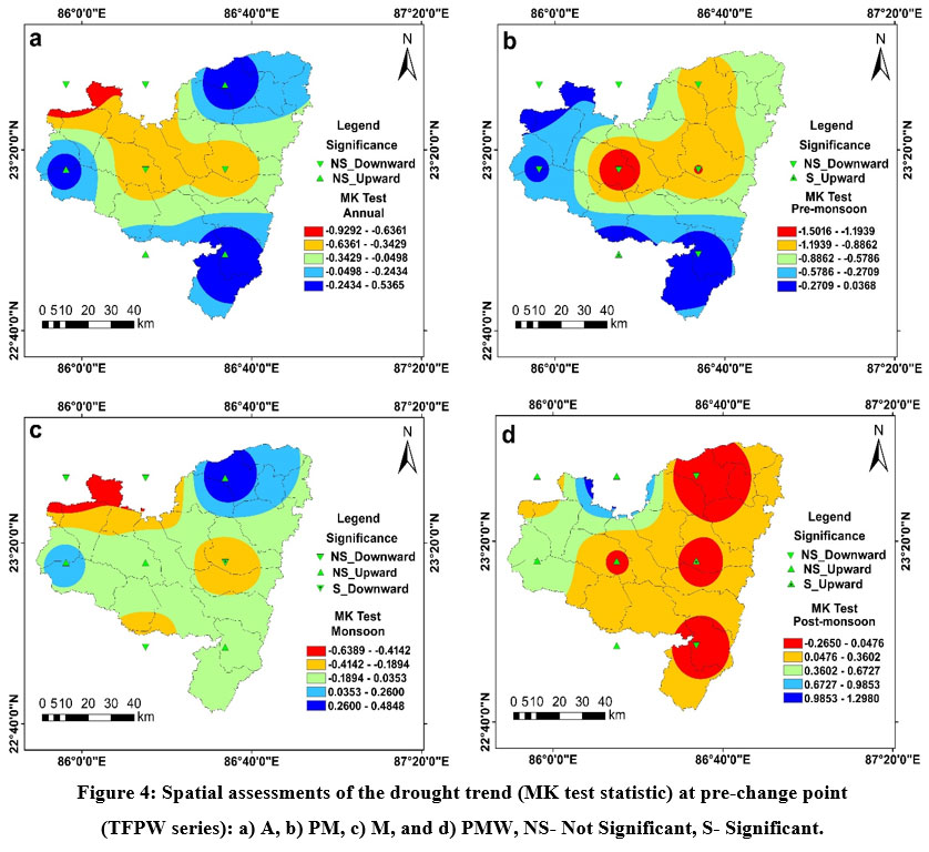
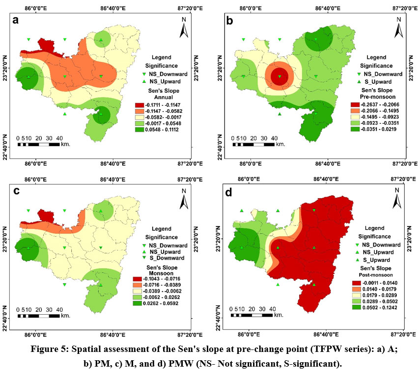
MK and Sen's slope were implemented on the TFPW series of droughts in both phases (i.e., before change point as well as the after-change point). Before the change point, for the annual series (A), MK test statistics varied from -0.9292 to 0.5365 (Fig. 4a), and Sen's slope fluctuated from -0.1711 to 0.1112 (Fig. 5a), respectively. Stations 229863 (1st station), 229866 (2nd Station), 233859 (3rd station), and 236866 (8th station) showed a non-significant upward trend, while stations 233863 (4th station), 233866 (5th station), 236859 (6th station), and 236863 (7th station) showed a non-significant downward trend. Generally, Western, southern, and north-eastern sections of the region were noticed with a non-significant upward drought trend. The remaining portions were identified with a non-significant downward trend of drought. Only meteorological station 229863 (1st Station) was noticed at the pre-monsoon phase (PM), with a significant upward trend. Other stations were noticed with a non-significant downward trend. At this phase, MK test statistic fluctuated from -1.5016 to 0.0368 (Fig. 4b) and Sen’s slope (Fig. 5b) varied from -0.2637 to 0.0219. At the monsoon phase (MS), MK test statistic and Sen's slope varied from -0.6389 to 0.4848 (Fig. 4c) and -0.1043 to 0.0592 (Fig. 5c). Only station 233866 (5th station) was noticed with a significant downward trend at this phase, and others were noticed with a non-significant upward or downward trend. North-Western portions were noticed with a downward trend at this phase, and north-eastern portions were noticed with an upward drought trend. At the post-monsoon phase (PMW), station 233866 (5th station) was observed with a significant upward trend, and other stations were noted with a non-significant upward or downward trend. Sen's slope and the MK test statistic at the post-monsoon period (PMW) fluctuated from -0.0011 to 0.1242 (Fig. 5d) and -0.2650 to 1.2980, respectively (Fig. 4d). At the post-monsoon period, the north-western regions were seen with a non-significant positive trend, while the north-eastern sections were marked with a non-significant negative trend of drought (PMW).
 | Figure 4: Spatial assessments of the drought trend (MK test statistic) at pre-change point (TFPW series): a) A, b) PM, c) M, and d) PMW, NS- Not Significant, S- Significant.
|
Source: Compiled by authors
 | Figure 5: Spatial assessment of the Sen's slope at pre-change point (TFPW series): a) A; b) PM, c) M, and d) PMW (NS- Not significant, S-significant).
|
Source: Compiled by authors
Status of drought at post-change point
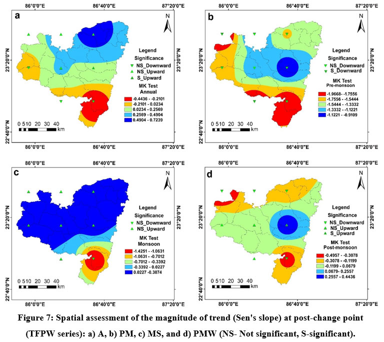
The MK test statistic and the Sen’s slope after the change (shift) point at the annual scale ranged between -0.4436 and 0.7239 (Fig. 6a) and -0.0149 and 0.0224 (Fig. 7a), respectively. In this case, only station 233866 (5th station) had a noticeable upward trend. There were other stations that had non-significant increasing or declining trends. North-eastern areas showed an in-significant upward trend, while south-west sections showed an in-significant declining trend. At the pre-monsoon phase (PM), MK test statistic (Fig. 6b) and Sen's slope (Fig. 7b) varied between -1.9688 to -0.9109 and -0.0397 to -0.0023 respectively. In this phase, a significant downward trend was observed at station 229863 (1st station). Other stations were noticed with a non-significant upward or downward trend. At the monsoon phase (MS), the study region was noticed with a non-significant negative (downward) or positive (upward) trend of drought. South-eastern portions were noticed with a non-significant downward trend, whereas the rest of the study region experienced a non-significant upward trend. At this phase, MK and Sen's slope varied between -1.4251 to 0.3847 (Fig. 6c) and -0.2637 to 0.0822 (Fig. 7c). At the post-monsoon phase (PMW), At station 233866 (5th station), there was a discernible rising trend. The southern and northern sections of this region marked a negligible downward trend. Significant rising (upward) trends in the drought were seen in the study region's eastern portions. Here, MK and Sen’s slope fluctuated from -0.4957 to 0.4436 (Fig. 6d) and -0.0122 to 0.0355 (Fig. 7d) respectively.
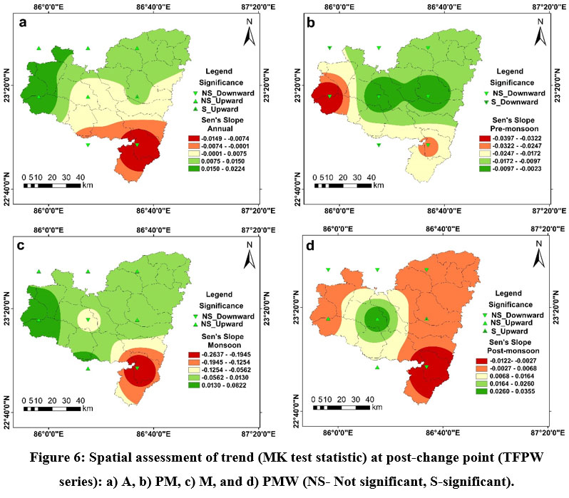 | Figure 6: Spatial assessment of trend (MK test statistic) at post-change point (TFPW series): a) A, b) PM, c) M, and d) PMW (NS- Not significant, S-significant).
|
Source: Compiled by authors
 | Figure 7: Spatial assessment of the magnitude of trend (Sen's slope) at post-change point (TFPW series): a) A, b) PM, c) MS, and d) PMW (NS- Not significant, S-significant).
|
Source: Compiled by authors
Percentage change assessment of drought
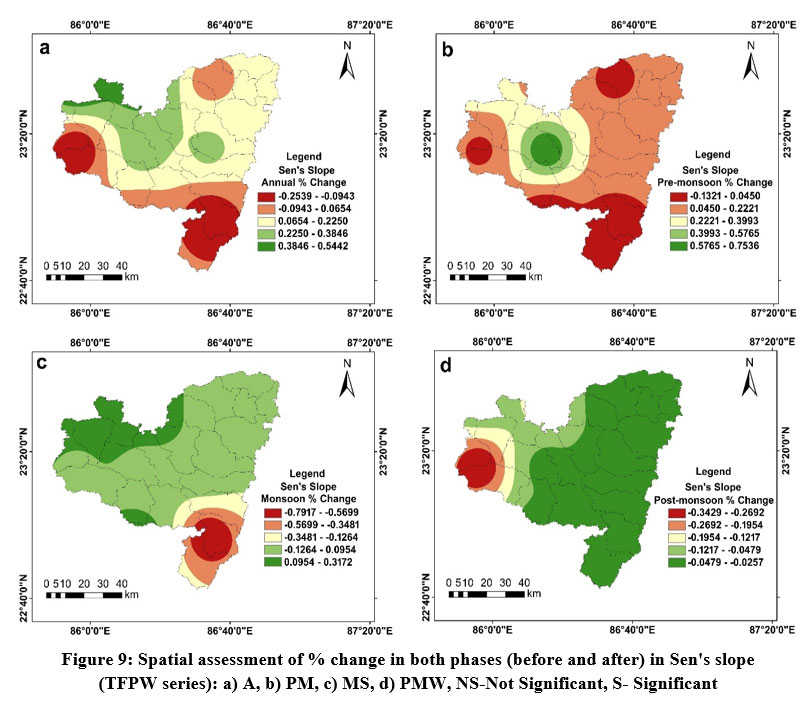
At the annual (A) and pre-monsoon phase (PM), the percentage change of drought was quite high in the eastern and middle sections of the region, and it was low in the southern and south-western sections of the Purulia. At the monsoon phase (MS), a percentage change of drought was observed as the lowest at the southern section; however, it was observed with a moderate to high nature for the remaining sections of the Purulia. The western part and also the northern sections of the study area experienced the lowest percentage change during the post-monsoon period (PMW). However, it was observed as the highest at the eastern sections of the region. At the annual scale, -2.8003% to 3.0323% (Fig. 8a) changes were observed for MK and -0.2539% to 0.5442% (Fig. 9a) changes were noticed for Sen’s slope. At the pre-monsoon phase (PM), -5.7246% to 1.0203% (Fig. 8b) changes were noticed for the MK and -0.1321% to 0.7536% (Fig. 9b) changes were observed for the Sen’s slope. At the monsoon phase (M), -4.1097% to 2.7957% (Fig. 8c) changes were identified for MK and -0.7917% to 0.3172% (Fig. 9c) changes were observed for the Sen’s slope. At post-monsoon phase, the change varied between -4.4416% to 1.2674% (Fig. 8d) for the MK and -0.3429% to -0.0257% (Fig. 9d) for the Sen’s slope. The highest negative change (%) at station 229863 (1st station) (-2.8%) and the highest positive change (%) at station 226863 (3.65%) were noted during the annual period (A). At the pre-monsoon phase, the largest negative change (%) (almost -5.7%) was noticed at stations 229863 (1st station), 229866 (2nd Station), and 236859 (6th station), and the highest positive change (%) (almost 1.02%) was noticed at the station 233863. At the monsoon season (M), the station 229863 (1st station) was noticed with the largest negative change (-4.11%) of drought, and station 236863 (7th station) was noticed with the highest positive change (3.53%). At the post-monsoon season, the highest negative change (-0.61%) was observed at station 236859 (6th station), and the largest positive change (0.04%) was found at station 233859 (3rd station).
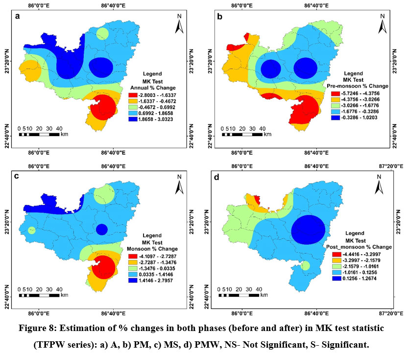 | Figure 8: Estimation of % changes in both phases (before and after) in MK test statistic (TFPW series): a) A, b) PM, c) MS, d) PMW, NS- Not Significant, S- Significant.
|
Source: Compiled by authors
 | Figure 9: Spatial assessment of % change in both phases (before and after) in Sen's slope (TFPW series): a) A, b) PM, c) MS, d) PMW, NS-Not Significant, S- Significant.
|
Source: Compiled by authors
The results of this research are analogous to the findings of other research conducted in same geographical locations. As of right now, 8 research articles were published on this region, to the best of our knowledge. Using the trends of SPI for 1971 and 2005, Palchaudhuri and Biswas85 assessed the spatiotemporal structure of the meteorological drought. The research explored that the northeast, northwest, and southwest regions of the district experience severe and extreme droughts. According to Bhunia et al.30, the Purulia have a high frequency of meteorological droughts. Using the exponential smoothing models, Shrestha et al.86 simulated the meteorological droughts of India using a bias corrected CMIP6 model and they found that the moderate drought is prevalent in these portions. Ghosh86 forecasted the drought conditions and discovered that moderate to severe droughts are likely to increase in upcoming days. Goswami38 analysed the monsoonal trend in meteorological drought of 1908 to 2009 and found that the central portions had faced comparatively high severity of drought. Drought was present in the Purulia's north-western, western, and north-eastern regions, according to Ghosh87, Bhardwaj88, Das89 and Mishra90. The eastern and south-western parts of the Purulia were identified by Bera et al.92 as the acute drought-prone portions. Using the exponential smoothing model, they made an effort to anticipate the drought and ultimately discovered the increasing nature of moderate and low droughts in this district. Low drought was anticipated in the Western portions of the region, while the moderate drought was anticipated in the Eastern sections. All of the research activities mentioned above are supported by the current study. It was found that the north-eastern, middle, and western regions of Purulia have a higher tendency of drought. The effects of the droughts on different regions have varying spatiotemporal sequences at different seasons 93,94. That spatiotemporal sequence can be easily identified by the change point. Moreover, consequences of the drought may vary in different phases and seasonal dimensions 95,96. Unfortunately, the research work mentioned above had not assessed the shifting nature of the drought (using the SPI). All of the research work abruptly identifies the drought in the Western and eastern portions of the Purulia. But the shifting nature of the drought from the Western to Eastern sections of the region is typically absent in research works done by the other researchers. The present research work meticulously identified the shifting nature of drought in the Purulia and therefore, this research became a mandatory and obvious read for the researchers.
Discussion
The trend of drought in the Purulia District matches with all Indian patterns. The possible causes of such drought trends in the Purulia have been deeply rooted within geo-environmental conditions such as the changing pattern of the climate. From 1990, the pattern of drought with the ENSO phenomenon has been changed and the relationship has been weakened97. The anomaly for the Walker and the surface temperatures are the root cause of such a changing realtionship98. So, alone ENSO event could not adequately explain the drought trend in the Indian context. On the broad perspective, the tendency of drought has increased at the eastern sections of the region, which typically depends on the local level factors, i.e., exhaustibility of the jet stream and weakening of meridional gradient induced by the SST99. The micro fluctuation of the meteorological variables at the eight precipitation sites is the focus of the Purulia drought trend study. As a result, the impact of ENSO and other events were not evaluated in this context. Instead, this research has essentially implied the local level factors, i.e., geology, relief, slope100, air pollution, changes of agricultural land use through the irrigated agriculture101, deforestation102 and rapid unplanned urbanization103. Originally belonging to a granitic terrain, the southern, north-eastern, and western portions of Purulia have crystalline basement rocks thinly covered by a mantle104,105. According to Nayak et al.106, due to the weathering of the fractured zones, and the porous structure of the rough dissected plateau, the soil of these sections cannot hold sufficient amount of water. According to Gupta and Patel107, a lower groundwater level in this area; exists due to a rugged and harsh topography. Hence, at pre and post-change points, the north-eastern, southern, and south-western portions are noticed with drought. Positive changes of trend dominate at the middle and eastern sections of the study region, indicating that the tendency of drought is increasing in these portions. The possible reasons for such a pattern are rapid urbanization, deforestation, and minimal scope of irrigation108.
Conclusion
Overall, the spatio-temporal variation of the drought trend was evaluated together with the change point at both the seasonal and yearly (annual) scales. The Sen's slope and Mann-Kendall test were used to calculate the drought trend. To find the most likely shifting (Change point) point in the time series, the Pettitt Mann-Whitney test was used to the annual and monthly scales. The best likely change point at seasonal and annual scales was between 1988 and 1989. Drought dominated at the southern, south-western, and north-eastern sections on a seasonal and annual scale (at both pre and post phases). But in the eastern parts of the territory, the shifting nature of the drought predominated in a positive direction.
In addition, the use of Morlet Wavelet transforms indicated that drought had a consistent periodicity that had ranged from 0.25 to 2 months by taking into account both yearly and seasonal scales. Due to the recent deterioration in the link between El-Nino and the Indian summer monsoon, this tendency was detected. A possible hint was given to local level elements such as the local-level geology, relief, slope, etc. which may be the responsible for such variances. Additionally, given that the Purulia depends on the production of agricultural crops, this research will have a big impact on agricultural planning that incorporates local level management of crop water. Consequently, the agricultural management plan of the Purulia would benefit from the findings of this research.
Acknowledgment
The authors are highly thankful to the CFSR website for providing free precipitation data to use in the manuscript.
Conflict of Interest
There is no conflict of interest/ competing interest exist.
Funding Sources
Authors receive no funding to do this research.
References
- Amrit, Kumar, Rajendra P. Pandey, and Surendra K. Mishra. Assessment of meteorological drought characteristics over Central India. Sustainable Water Resources Management. 2018; 4: 999-1010.
- Khadr, Mosaad. Forecasting of meteorological drought using Hidden Markov Model (case study: The upper Blue Nile river basin, Ethiopia). Ain Shams Engineering Journal .2016;7(1): 47-56.
- Beier, Claus, et al. Precipitation manipulation experiments–challenges and recommendations for the future. Ecology letters.2012; 15(8): 899-911.
- Salehnia, Nasrin, et al. Estimation of meteorological drought indices based on AgMERRA precipitation data and station-observed precipitation data. J Arid Land. 2017; 9: 797-809.
- Wang, L. N., et al. The drought trend and its relationship with rainfall intensity in the Loess Plateau of China. Nat Hazards. 2015; 77: 479-495.
- Mishra, Ashok K., and Vijay P. Singh. A review of drought concepts. J Hydrol. 2010; 391.1(2): 202-216.
- Mishra, Prabhat Kumar, et al. Production analysis of composite fish culture in drought prone areas of Purulia: The implication of financial constraint. Aquaculture. 2022; 548: 737629.
- Spinoni, Jonathan, et al. A new global database of meteorological drought events from 1951 to 2016. Journal of Hydrology: Regional Studies. 2019; 22: 100593.
- Abbasian, Mohammad Sadegh, Mohammad Reza Najafi, and Ahmad Abrishamchi. Increasing risk of meteorological drought in the Lake Urmia basin under climate change: Introducing the precipitation–temperature deciles index. J Hydrol. 2021;592: 125586.
- Pandey, Varsha, et al. Multi-satellite precipitation products for meteorological drought assessment and forecasting in Central India. Geocarto Int. 2022; 37(7): 1899-1918.
- Datta, Rajarshi, Abhishek A. Pathak, and B. M. Dodamani. Assessment of meteorological drought return periods over a temporal rainfall change. Trends in Civil Engineering and Challenges for Sustainability: Select Proceedings of CTCS 2019. 2021: 573-592.
- Bisht, Deepak Singh, et al. Drought characterization over India under projected climate scenario. Int J Climatol. 2019; 39(4): 1889-1911.
- Kar, B., J. Saha, and J. D. Saha. Analysis of meteorological drought: the scenario of West Bengal. Indian Journal of Spatial Science. 2012; 3(2): 1-11.
- Kundu, Suman Kumar, and Tarun Kumar Mondal. Analysis of long-term rainfall trends and change point in West Bengal, India. Theor Appl Climatol. 2019; 138: 1647-1666.
- Guttman, Nathaniel B. Comparing the palmer drought index and the standardized precipitation index 1. JAWRA. 1998; 34(1): 113-121.
- Mega, Nabil, and Abderrahmane Medjerab. Statistical comparison between the standardized precipitation index and the standardized precipitation drought index. Modeling Earth Systems and Environment. 2021;7: 373-388.
- Cheval, Sorin, et al. Spatiotemporal variability of meteorological drought in Romania using the standardized precipitation index (SPI). Clim Res. 2014; 60(3): 235-248.
- Awchi, Taymoor A., and Maad M. Kalyana. Meteorological drought analysis in northern Iraq using SPI and GIS. Sustainable Water Resources Management .2017;3: 451-463.
- Wu, Hong, et al. An evaluation of the Standardized Precipitation Index, the China?Z Index and the statistical Z?Score. Int J Climatol. 2001; 21(6): 745-758.
- World Meteorological Organization. Standardized precipitation index user guide. 2012. ISBN 978-92-63-11091-6. 16p.
- Han, Eunjin, and Amor VM Ines. Downscaling probabilistic seasonal climate forecasts for decision support in agriculture: A comparison of parametric and non-parametric approach. Climate Risk Management. 2017;18: 51-65.
- Mahajan, D. R., and B. M. Dodamani. Trend analysis of drought events over upper Krishna basin in Maharashtra. Aquat Pr. 2015; 4: 1250-1257.
- Sharma, Ashutosh, and Manish Kumar Goyal. Assessment of drought trend and variability in India using wavelet transform. Hydrolog Sci J .2020; 65(9): 1539-1554.
- Vishwakarma, Ankur, Mahendra Kumar Choudhary, and Mrityunjay Singh Chauhan. Applicability of SPI and RDI for forthcoming drought events: a non-parametric trend and one-way ANOVA approach. J Water Clim Change. 2020; 11(S1): 18-28.
- Bhunia, Prasenjit, Pritha Das, and Ramkrishna Maiti. Meteorological drought study through SPI in three drought prone districts of West Bengal, India. Earth Systems and Environment. 2020; 4(1): 43-55.
- Das, Prabir Kumar, et al. Trends and behaviour of meteorological drought (1901–2008) over Indian region using standardized precipitation–evapotranspiration index. Int J Climatol. 2016; 36(2): 909-916.
- Naresh Kumar, M., et al. Spatiotemporal analysis of meteorological drought variability in the Indian region using standardized precipitation index. Meteorol Appl. 2012. 19(2): 256-264.
- Shikary, Chumki, and Somnath Rudra. Measuring urban land use change and sprawl using geospatial techniques: A study on Purulia Municipality, West Bengal, India. IJRAR. 2021;6(1). 819-829.
- Ghosh, Prasanta Kumar, Sujay Bandyopadhyay, and Narayan Chandra Jana. Mapping of groundwater potential zones in hard rock terrain using geoinformatics: a case of Kumari watershed in western part of West Bengal. Modeling Earth Systems and Environment. 2016; 2: 1-12.
- Singha, A., Pramanick, N., and Acharyya, R. Implication of Applying IPCC AR4 and AR5 Framework for Drought-based Vulnerability and Risk Assessment in Bankura and Purulia Districts, West Bengal. In IOP Conference Series: Earth and Environmental Science. IOP Publishing. 2023; 1164(1). 012009.
- SAFE. Community-ecosystem approach for adaptive watershed management in drought-prone tribal areas of West Bengal. 2011. www.resourceaward.org.
- Ghosh, Prasanta Kumar, and Narayan Chandra Jana. Groundwater potentiality of the Kumari River Basin in drought-prone Purulia upland, Eastern India: a combined approach using quantitative geomorphology and GIS. Sustainable Water Resources Management. 2018; 4: 583-599.
- Adhikari, P., D. Sen, and N. Uphoff. System of Rice Intensification as a resource-conserving methodology: contributing to food security in an era of climate change. SATSA: State Agricultural Technologists Service Association, West Bengal, India. Annual Technical. 2010; 14: 26-44.
- Thakur, Amod K., and Norman T. Uphoff. How the system of rice intensification can contribute to climate?smart agriculture. Agronomy Journal .2017;109(4): 1163-1182.
- Banik, Pabitra, Abhyudy Mandal, and M. Sayedur Rahman. Markov chain analysis of weekly rainfall data in determining drought-proneness. Discrete Dyn Nat Soc. 2002; 7(4): 231-239.
- Singh, P. K., et al. Spatial analysis of rainfall variability and rainfed rice crop using GIS Technique in West Bengal (India). MAUSAM. 2017; 68(2): 287-298.
- Mandal, Biplab, Gour Dolui, and Sujan Satpathy. Land suitability assessment for potential surface irrigation of river catchment for irrigation development in Kansai watershed, Purulia, West Bengal, India. Sustainable Water Resources Management. 2018; 4: 699-714.
- Goswami, Asutosh. Identifying the trend of meteorological drought in Purulia district of West Bengal, India. Environment and Ecology. 2019; 37(1B): 387-392.
- Census of India. 2011): Available at https://censusindia.gov.in/census.website/.
- Biswas, Sudipta, and Sukumar Pal. Tribal Land Rights: A Situational Analysis in the Context of West Bengal. Journal of Land and Rural Studies. 2021; 9(1): 193-209.
- Ghosh, Bhola Nath, and Utpal Kumar De. Land Acquisition in Singur for Industrialization: SEZ. Politics and Economic Intricacy. 2016.
- Roy, A. K., et al. System of Rice Intensification (SRI): An Experiment in Purulia Under NAIP. Environment and Ecology. 2012; 30(4): 1280-1284.
- Cornish, Peter S., et al. Improving crop production for food security and improved livelihoods on the East India Plateau II. Crop options, alternative cropping systems and capacity building. Agr Syst. 2015; 137: 180-190.
- Palchaudhuri, Moumita, and Sujata Biswas. Application of AHP with GIS in drought risk assessment for Puruliya district, India. Nat Hazards. 2016; 84: 1905-1920.
- Climate Forecast System Reanalysis dataset obtained from https://swat.tamu.edu/data/cfsr website.
- Sommerlot, Andrew Richard. Coupling Physical and Machine Learning Models with High Resolution Information Transfer and Rapid Update Frameworks for Environmental Applications. Diss. Virginia Tech. 2017.
- Sehgal, Vinit, and Venkataramana Sridhar. Watershed-scale retrospective drought analysis and seasonal forecasting using multi-layer, high-resolution simulated soil moisture for Southeastern US. Weather and Climate Extremes. 2019. 23: 100191.
- Dile, Yihun Taddele, and Raghavan Srinivasan. Evaluation of CFSR climate data for hydrologic prediction in data?scarce watersheds: an application in the Blue Nile River Basin. JAWRA Journal of the American Water Resources Association. 2014; 50(5): 1226-1241.
- Yihdego, Yohannes, Babak Vaheddoost, and Radwan A. Al-Weshah. Drought indices and indicators revisited. Arab J Geosci. 2019; 12(69): 1-12.
- Li, Lingcheng, et al. Elucidating diverse drought characteristics from two meteorological drought indices (SPI and SPEI) in China. Journal of Hydrometeorology. 2020. 21(7): 1513-1530.
- McKee, Thomas B., Nolan J. Doesken, and John Kleist. The relationship of drought frequency and duration to time scales. Proceedings of the 8th Conference on Applied Climatology. 1993; 17(22).
- Edwards, Daniel C. Characteristics of 20th Century drought in the United States at multiple time scales. Air Force Inst of Tech Wright-Patterson Afb Oh, 1997; 155.
- Sönmez, F. Kemal, et al. An analysis of spatial and temporal dimension of drought vulnerability in Turkey using the standardized precipitation index. Nat Hazards. 2005; 35(2): 243-264.
- Thom, Herbert CS. A note on the gamma distribution. Mon Weather Rev. 1958; 86(4): 117-122.
- AGRIMETSOFT. Meteorological Drought Monitor (Version 1) [Computer software]. 2017; Available at: https://agrimetsoft.com/MDM.aspx.
- Nikzad Tehrani, E., H. Sahour, and M. J. Booij. Trend analysis of hydro-climatic variables in the north of Iran. Theor Appl Climatol. 2019. 136(1): 85-97.
- Tosunoglu, F., and O. Kisi. Trend analysis of maximum hydrologic drought variables using Mann–Kendall and ?en's innovative trend method. River Res Appl. 2017. 33(4): 597-610.
- Abeysingha, N. S., and U. R. L. N. Rajapaksha. SPI-based spatiotemporal drought over Sri Lanka. Adv Meteorol. 2020. 2020.
- Mann H.B. Non-parametric tests against trend. Econometrica. 1945; 13:245–259.
- Kendall M. Rank correlation methods, 4th edn. 1945. Charles Griffin, London.
- Huang, Shengzhi, et al. Spatio-temporal changes and frequency analysis of drought in the Wei River Basin, China. Water Resour Manag. 28; 2014: 3095-3110.
- Ali, R. O., Abubaker, S. R. Trend analysis using Mann-Kendall, Sen's slope estimator test and innovative trend analysis method in Yangtze River basin, China. International Journal of Engineering & Technology. 2019;8(2): 110-119.
- Gajbhiye, Sarita, et al. Precipitation trend analysis of Sindh River basin, India, from 102?year record (1901–2002). Atmos Sci Lett. 2016;17(1):71-77.
- Theil, Henri. A rank-invariant method of linear and polynomial regression analysis. Indagationes Mathematicae 1950;12(85): 173.
- Sen, Pranab Kumar. Estimates of the regression coefficient based on Kendall's tau. Journal of the American Statistical Association. 1968;63(324): 1379-1389.
- Tabari, Hossein, et al. Shift changes and monotonic trends in autocorrelated temperature series over Iran. Theor Appl Climatol .2011.109: 95-108.
- Serinaldi, Francesco, and Chris G. Kilsby. Stationarity is undead: Uncertainty dominates the distribution of extremes. Adv Water Resour. 2015. 77: 17-36.
- Von Storch, Hans. Misuses of statistical analysis in climate research. Analysis of Climate Variability: Applications of Statistical Techniques Proceedings of an Autumn School Organized by the Commission of the European Community on Elba from October 30 to November 6, 1993. Springer Berlin Heidelberg. 1999; 11-26.
- Tabari, Hossein, Behzad Shifteh Somee0, and Mehdi Rezaeian Zadeh. Testing for long-term trends in climatic variables in Iran. Atmos Res.2011a;100(1): 132-140.
- ?en, Zekâi. Hydrological trend analysis with innovative and over-whitening procedures. Hydrolog Sci J. 2017;62(2): 294-305.
- Yue, Sheng, et al. The influence of autocorrelation on the ability to detect trend in hydrological series. Hydrol Process. 2002;16(9): 1807-1829.
- Tabari, Hossein, and P. Hosseinzadeh Talaee. Analysis of trends in temperature data in arid and semi-arid regions of Iran. Global Planet Change. 2011b;79(1-2): 1-10.
- ?en, Zekâi. Innovative trend analysis methodology. Journal of Hydrologic Engineering. 2012. 17(9): 1042-1046.
- Partal, Turgay, and Özgür Ki?i. Wavelet and neuro-fuzzy conjunction model for precipitation forecasting. J Hydrol. 2007;342(1-2): 199-212.
- Grossmann, Alexander, and Jean Morlet. Decomposition of Hardy functions into square integrable wavelets of constant shape. SIAM Journal on Mathematical Analysis. 1984;15(4): 723-736.
- Araghi, Alireza, et al. Using wavelet transforms to estimate surface temperature trends and dominant periodicities in Iran based on gridded reanalysis data. Atmos Res. 2015;155: 52-72.
- Liu, Dedi, et al. Analysis of trends of annual and seasonal precipitation from 1956 to 2000 in Guangdong Province, China. Hydrolog Sci J. 2012;57(2): 358-369.
- Morlet, Jean, et al. Wave propagation and sampling theory—Part I: Complex signal and scattering in multilayered media. Geophysics. 1982;47(2): 203-221.
- Torrence, Christopher, and Gilbert P. Compo. A practical guide to wavelet analysis. Bulletin of the American Meteorological society. 1998;79(1): 61-78.
- Rösch, Angi, and Harald Schmidbauer. WaveletComp 1.1: A guided tour through the R package. 2014. URL: http://www. hsstat. com/projects/WaveletComp/WaveletComp_guided_tour. pdf.
- Pingale, Santosh M., et al. Trend analysis of climatic variables in an arid and semi-arid region of the Ajmer District, Rajasthan, India. Journal of Water and Land Development. 2016;28(1): 3.
- Kruskal, William H., and W. Allen Wallis. Use of ranks in one-criterion variance analysis. Journal of the American statistical Association. 1952;47(260): 583-621.
- Yu, Pao-Shan, Tao-Chang Yang, and Chun-Chao Kuo. Evaluating long-term trends in annual and seasonal precipitation in Taiwan. Water Resour Manage. 2006; 20 (6): 1007-1023.
- Zhang, Ling, and Kun Han. How to analyze change from baseline: absolute or percentage change. D-level Essay in Statistics. Dalarna, Sweden: Dalarna University.
- Palchaudhuri, Moumita, and Sujata Biswas. Analysis of meteorological drought using Standardized Precipitation Index–A case study of Puruliya district, West Bengal, India. International Journal of Environmental and Ecological Engineering. 2013; 7(3): 167-174.
- Shrestha, Alen, et al. Climatological drought forecasting using bias corrected CMIP6 climate data: A case study for India. Forecasting. 2020. 2(2): 59-84.
- Ghosh, Krishna Gopal. Spatial and temporal appraisal of drought jeopardy over the Gangetic West Bengal, eastern India. Geoenvironmental Disasters. 2019. 6: 1-21.
- Bhardwaj, Kunal, et al. Propagation of meteorological to hydrological droughts in India. J Geophys Res: Atmos. 2020;125(22): e2020JD033455.
- Das, Prabir Kumar, Abhishek Chakraborty, and Mullapudi VR Seshasai. Spatial analysis of temporal trend of rainfall and rainy days during the Indian Summer Monsoon season using daily gridded (0.5× 0.5) rainfall data for the period of 1971–2005. Meteorol Appl. 2014; 21(3): 481-493.
- Mishra, S. Drought and its management in West Bengal. Indian Journal of Landscape and Ecological Studies. 2006; 35(1):20—28.
- Mishra, S. Climate change and adaptation strategy in Agriculture—a West Bengal scenario. Geog Rev Ind. 2012;74: 21-31.
- Bera, Biswajit, et al. Trends and variability of drought in the extended part of Chhota Nagpur plateau (Singbhum Protocontinent), India applying SPI and SPEI indices. Environmental Challenges. 2021; 5: 100310.
- Xu, Kai, et al. Spatio-temporal variation of drought in China during 1961–2012: A climatic perspective. J Hydrol. 2015;526: 253-264.
- Wang, Fei, et al. Capability of remotely sensed drought indices for representing the spatio–temporal variations of the meteorological droughts in the Yellow River Basin. Remote Sens-Basel. 2018;10(11): 1834.
- Daryanto, Stefani, Lixin Wang, and Pierre-André Jacinthe. Global synthesis of drought effects on maize and wheat production. PloS one. 2016;11(5): e0156362.
- Doughty, Christopher E., et al. Drought impact on forest carbon dynamics and fluxes in Amazonia. Nature. 2015;519(7541): 78-82.
- Mondal, Arun, Deepak Khare, and Sananda Kundu. Spatial and temporal analysis of rainfall and temperature trend of India. Theor Appl Climatol. 2015;122: 143-158.
- Kumar, K. Krishna, Balaji Rajagopalan, and Mark A. Cane. On the weakening relationship between the Indian monsoon and ENSO. Science.1999;284(5423): 2156-2159.
- Naidu, C. V., et al. Is summer monsoon rainfall decreasing over India in the global warming era? Journal of Geophysical Research: Atmospheres. 2009;114(D24). 1-16.
- Basist, Alan, Gerald D. Bell, and Vernon Meentemeyer. Statistical relationships between topography and precipitation patterns. J Climate. 1994;7(9): 1305-1315.
- Douglas, Ellen M., et al. Changes in moisture and energy fluxes due to agricultural land use and irrigation in the Indian Monsoon Belt. Geophys Res Lett.2006. 33(14):1-5
- Nair, Udaysankar S., et al. Impact of land use on Costa Rican tropical montane cloud forests: Sensitivity of cumulus cloud field characteristics to lowland deforestation. J Geophys Res: Atmos. 2003;108(D7):1-13.
- Sadashivam, T., and Shahla Tabassu. Trends of urbanization in India: issues and challenges in the 21st century. International Journal of Information Research and Review. 2016; 3(5): 2375-2384.
- Nag, S. K., and P. Ghosh. Variation in groundwater levels and water quality in Chhatna Block, Bankura District, West Bengal—A GIS approach. J Geol Soc India. 2013; 81: 261-280.
- Dolui, Gour, et al. Multi-criteria Decision-Making Approach Using Remote Sensing and GIS for Assessment of Groundwater Resources. Geostatistics and Geospatial Technologies for Groundwater Resources in India; 2021: 59-79.
- Nayak, Siperna, et al. Structural control on the occurrence of groundwater in granite gneissic terrain, Purulia, West Bengal. Arab J Geosci; 2020; 13(18): 1-14.
- Gupta, Devarupa, and Priyank Pravin Patel. Mapping groundwater level fluctuation and utilisation in Puruliya District, West Bengal. Geostatistics and geospatial technologies for groundwater resources in India. 2021: 413-442.
- Shikary, Chumki, and Somnath Rudra. Measuring urban land use change and sprawl using geospatial techniques: A study on Purulia Municipality, West Bengal, India. Journal of the Indian Society of Remote Sensing. 2021; 49: 433-448.


