Optimization of Grey Water Characteristics Using Electrocoagulation and Response Surface Methodology
Charlotte Mashiya Rajesh1
*
 , Ravathi Mohanadas Chandrika2
and Revathi Sampath Kumar2
, Ravathi Mohanadas Chandrika2
and Revathi Sampath Kumar2
1
Department of Environmental Engineering,
Government college of technology,
Anna university,
Coimbatore,
Tamil Nadu
India
2
Department of Civil Engineering,
Government college of technology,
Anna university,
Coimbatore,
Tamil Nadu
India
http://dx.doi.org/10.12944/CWE.20.2.16
Copy the following to cite this article:
Rajesh C. M, Chandrika R. M, Kumar R. S. Optimization of Grey Water Characteristics Using Electrocoagulation and Response Surface Methodology.Curr World Environ 2025;20(2). DOI:http://dx.doi.org/10.12944/CWE.20.2.16
Copy the following to cite this URL:
Rajesh C. M, Chandrika R. M, Kumar R. S. Optimization of Grey Water Characteristics Using Electrocoagulation and Response Surface Methodology.Curr World Environ 2025;20(2).
Download article (pdf)
Citation Manager
Publish History

Introduction
Grey water describes the relatively clean, researchers like Pushparaj, Shubhi Gupta and Prasenjit Mondal,1 emphasize that wastewater which comes from sinks, bathtubs and washing machines and other kitchen appliances, compared to black water (which includes toilet waste), it usually has fewer impurities and makes up a sizable amount of household waste water. Given its makeup, grey water has a substantial opportunity exists for product recycling and restage functions2; as well as for meeting water demands in areas with limited supplies. The grey water from home waste sullage, can be processed and used as a ground water recharge mechanism. In order to address water scarcity by another investigation3 reusing of recycled water sources must be taken to raise the dried-up riverine zones.
Need for This Study
Grey water constitutes approximately 30- 50% of the waste water that is released into sewer systems. Although treated grey water is unlikely to be safe for consumption, its recycling can lead to substantial reductions in water expenses for businesses. The release of untreated grey water contributes to groundwater contamination through the introduction of nutrients and micro-pollutants, as well as causing eutrophication in surface water bodies. The conversion of agricultural byproducts into activated carbon presents both economic and environmental benefits.4-5 the grey water can be reused by electrocoagulation method by using suitable adsorbent.
Materials and Methods
Collection of Raw Material
Plantain fruit bracts were collected from local community market at Coimbatore which is considered as a waste material.
Electrocoagulation Unit
The unit simply comprises of the choice electrode placed within a distance of 5 cm using a thermocol or cardboard sheet where it is placed in a container filled with grey water and the ends of the electrode is kept immersed in the water such that to remove the contaminants during the process.6
Preparation
Researchers washed bracts with distilled water to eliminate dust and maintained them under 37°C sun exposure for four days of drying.7 The Grey water is filtered as pre-treatment before actual coagulation.
Synthesis and activation
The obtained charcoal is cooled down and divided into three parts, mixed with Phosphoric acid, Potassium hydroxide, Calcium Carbonate.
The obtained charcoal is cooled down and divided into three parts, the ratio of 1:2 (1g: carbon substitute (Banana Bract); 2g:1+1 distilled water + acid (say Phosphoric acid and respectively))
The activation is done using,
H3PO4 (Phosphoric Acid) Phosphorous is chosen due to excellent synthesis process lead to high pore volume and increase in diameter for perfect adsorption.
CaCo3 (Calcium Carbonate) is chosen for pore structure development, the decomposition of CaO+Co2 this release creates pores in carbon structure extreme area.
KOH (potassium hydroxide) is chosen for adsorption capacity and reduced activating temperature and high pore formation (reaction between KOH and carbon generates gases that creates and expand pore network. A crucible received 1-hour exposure at 400 °C within the muffle furnace. The device was left to cool before being transferred into an air-tight package for subsequent testing.
Treatment by Electro-coagulation
500ml of sample in filled accurately in two beakers and 0.5g (since it’s the threshold for effective coagulation) of activated carbon (AC) is added respectively in separate beakers.
Mixed uniformly by using a Magnetic stirrer for approximately 3 minutes.
The positive and negative electrodes were connected to 2 Aluminum (Al) strips (say for first process) with a spacing of 5cm from each electrode and a supply of 12.9v DC power source.
The supplication is maintained undisturbed for 30 minutes and simultaneously for 60 and 90 minutes. after the period of time the metal ions get trapped on electrode surface and suspended particles form flocs and can be removed by simple filtration process. This process is repeated for different electrodes and adsorbent likewise.
Electrode Selection
Aluminum is Best for removing turbidity and color. Copper can be used For pH greater than 7, copper ions produce Cu(OH)2 and CuO, which can act as coagulants. Stainless steel is Best for removing total chromium in waste water source.
Selection of activation agent Calcium carbonate
Flexible porous structure and functional group modification increases the pore space in adsorbent.
Phosphoric Acid
Creates the porous structure, protects the carbon skeleton, creates enriched functional groups in adsorbents.
It causes less equipment corrosion.
Potassium Hydroxide
Creates large surface area narrow porosity distribution in adsorbents.
Results
The physio chemical analysis of effluent showed that the effluent is slightly alkaline in nature with less Dissolved oxygen and has high turbidity. If this water is discharged without treatment, it will pose a threat to Ground water. Though turbidity levels were high as compared to standards, their levels were not so much high. (Refer Table 1). Therefore, it’s safe to discharge into ground and can help to increase ground water table and reduce scarcity of water and can be used in some industrial purposes (oil refineries, coolants, etc.,).
Table 1: Initial Physico-chemical parameters of Grey water
Sl. No | Parameters | Effluent Sample | Standard of EPA* |
1 | pH | 8.28 | 6.5-8.5 mg/l |
2 | Temperature | 28o C | 20-35o C |
3 | Turbidity | 49.8 NTU | < 5 NTU |
4 | COD | 1250 mg/l | <100 mg/l |
5 | Dissolved oxygen | 4.2 mg /l | 2.7-5.2 mg/l |
6 | Hardness | 310 mg /l | 50-150 mg /l |
7 | Total dissolved solids | 1850 mg /l | 500-1000mg/l |
* These ranges are based on general standards and guidelines from the EPA and state/local regulations this confirms that the post-treatment range should be within the mentioned range from standard of EPA. The third column represents the initial concentration of pollutants present in the sample.
Characteristics of adsorbent
X-Ray Diffraction
Phosphoric Acid
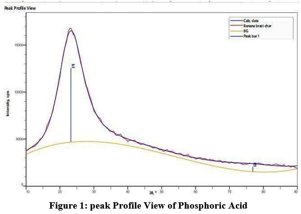
Peak is observed at 23.22 with miller index (1 0 1) shown in figure 1. The XRD peak with 20 values 23.22 corresponds to the miller index (1 0 1) The prepared crystalline structure was estimated as, D=16.95 nm. using Braggs’s law, d=0.382 nm Inner planar spacing is calculated.
 |
|
Potassium Hydroxide
Peak is observed at 28.48. In the observed pattern its depicted in figure 2,The XRD peak with 20 values 28.48 is The prepared crystalline structure was estimated as, D=17.13 nm. Inner planar spacing is calculated using Braggs’s law, d=0.31 nm.
Calcium Carbonate
Peak is observed at 31.73. In the observed pattern, The XRD peak with 20 value 31.73 has The prepared crystalline structure was estimated as, D=17.26 nm,Inner planar spacing is calculated Braggs’s law,d=0.28 nm. The peak is shown in figure 3.
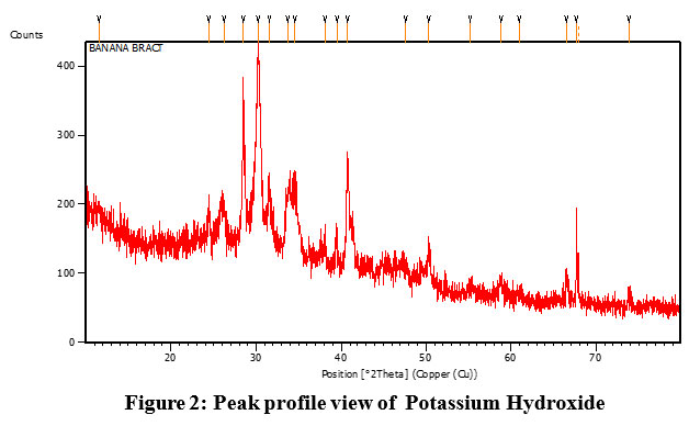 | Figure 2: Peak profile view of Potassium Hydroxide
|
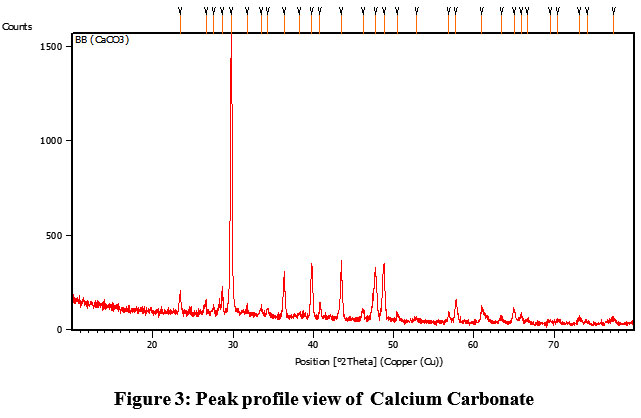 | Figure 3: Peak profile view of Calcium Carbonate
|
Fourier Transform Infra red Spectroscopy
Phosphoric Acid
6
Potassium Hydroxide
The FTIR spectrum of the broad peak at 3628.58 cm-1 which is depicted in figure 5 corresponds to the O-H stretching vibration of the alcohol group. (medium, sharp peak).9 The peak at 2560.06 cm-1 corresponds to the O-H stretching carboxylic acid class with strong, broad peak.
Calcium Carbonate
The FTIR spectrum of the broad peak at 3520 cm-1 which is depicted in figure 6 corresponds to the primary amine.11 (Medium peak).The peak at 2515.32 cm-1 corresponds to the O- H stretching carboxylic acid class with strong, broad peak.The peak at 1493.03 cm-1 corresponds to the nitro compound group with strong peak.11 The peak at 709.71cm-1 corresponds to the C=C bending alkene with strong peak.11
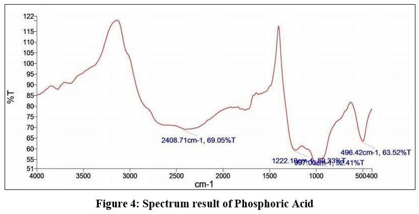 | Figure 4: Spectrum result of Phosphoric Acid
|
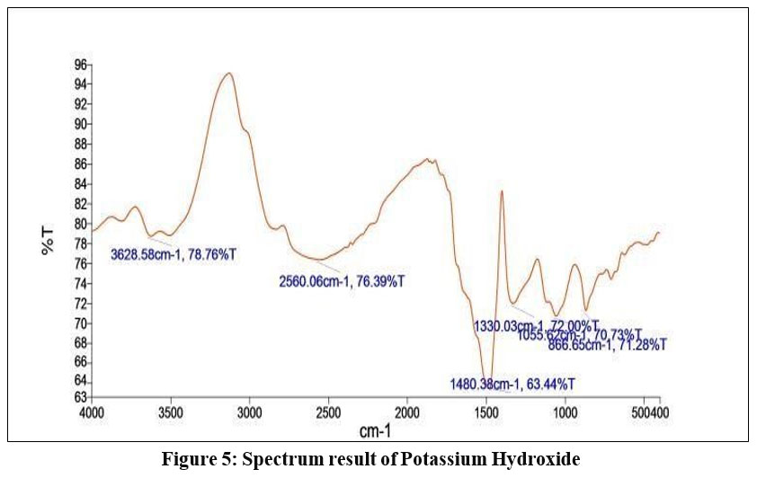 | Figure 5: Spectrum result of Potassium Hydroxide
|
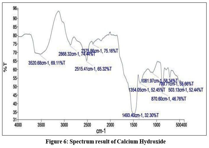 | Figure 6: Spectrum result of Calcium Hydroxide
|
Scanning Electron Microscope
Morphological Analysis of Activated Carbon (Calcium Carbonate)
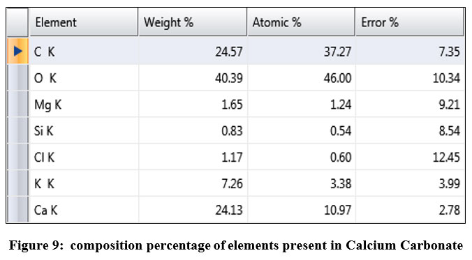
Morphological analysis was performed in order to study the structure, elemental composition, thickness, grain size of sample material. SEM and EDAX were performed. SEM analysis was done using TESCAN MIRA3 Fe-SEM equipment. From SEM images, it was found that obtained activated carbon is smooth with glossy surface but irregular in shape. The fibrous structure may be due to helically wound cellulose microfibrils in an amorphous matrix of lignin and cellulose. Large pores were created due to the thermal decomposition of these phloem fibers. Such this structure provides high adsorption property to the adsorbent. EDAX mainly done to find the elemental composition of adsorbent. EDAM was done using EDAX-APEX software. From EDAX image, it was observed that adsorbent contains major element of carbon, potassium and calcium around 88% from figure 9. along with that a negligible number of other elements are present. Is shown in figure 7 and 8. Particle size of the adsorbent varied from 133 um to 19.5 um with a surface area.
This clearly shows that the pores are of sufficient size to adsorb contaminants.
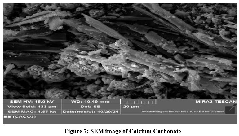 | Figure 7: SEM image of Calcium Carbonate
|
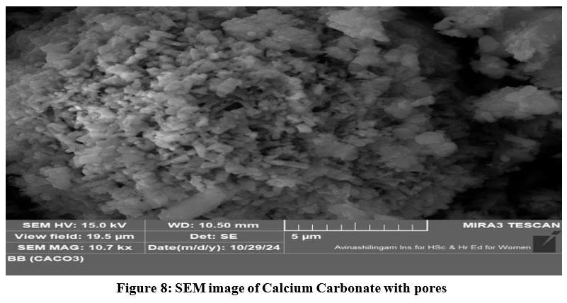 | Figure 8: SEM image of Calcium Carbonate with pores
|
 | Figure 9: composition percentage of elements present in Calcium Carbonate
|
Optimization Using RSM
The RSM optimizes the results within a limited runs given in figure 10, the build information is mentioned in table 2.
Table 2: Build Information of RSM
File Version | 23.1.6.0 |
Design Type | Response Surface |
Study Type | Box Behnken |
Sub Type | Randomized |
Runs | 17 |
Design Model | Quadratic |
Build Time | 89.00 |
Significance of Box-Benkhen Type
By employing Box-Benkhen designs manufacturers generate complex response surfaces through fewer experimental runs than standard factorial approaches require. The final and actual values obtained are given in table 3 and 4, the confirmation run is stipulated in figure 17. The A,B,C represents time, electrode and activated carbon respectively.
Table 3: Equations in terms of Coded
EQUATIONS IN TERMS OF CODED | |
Turbidity | 12.70+0.8250XA+0.3125XB+1.21XC+1.45XAB- 1.25XAC+2.07XBC+12.59XA2+9.26XB2+14.31XC2 |
TDS | 940+5XA+0XB+10XC+32.50XAB- 12.50 XAC+32.50XBC+121.25XA2+76.25XB2+136.25XC2 |
Hardness | 110+2.50XA+7.50XB+10XC+20XAB-10XAC+35XBC+77.50XA2+32.50XB2+82.50XC2 |
DO | 2.80+0.05XA+0.025XB-0.025XC+0.05XAB+0.05XAC+0XBC+0.55XA2+0.60XB2+0.70XC2 |
COD | 750+28.75XA-3.50XB+25.25XC+57.50XAB- 25XAC+49.50XBC+184XA2+108.50XB2+241XC2 |
pH | 2.65+0.0443XA-0.0443XB-0.0429XC+0.0457XAB- 0.0429XAC+0.0429XBC+0.0685XA2+0.0685XB2+0.157XC2 |
Table 4: Equations in actual factors
EQUATIONS IN TERMS OF ACTUAL FACTORS | |
Turbidity | +61.4-1.65 time-2.58 electrode +1.85 activation agent+0.048 time*electrode-0.02 time* activation agent +1.03 electrode *activation agent +0.013 time2 +0.013 electrode2 +34.06 activation agent2 |
TDS | +1415-16 time-65 electrode +17.5 activation agent +1.083 time*electrode-0.2083 time* activation agent + 16.25 electrode *activation agent +0.134722 time2 + 9.26 electrode2 +3.57 activation agent2 |
Hardness | +415-10.25 time-32.5 electrode +15activation agent +0.6 time*electrode-0.16 time* activation agent +17.5 electrode *activation agent + 0.086 time2 + 32.5 electrode2 +20.62 activation agent2 |
DO | +4.9-0.07 time-0.075 electrode -0.062activation agent +0.001 time*electrode +0.00083 time* activation agent -2.07 electrode *activation agent + 0.0006 time2 + 0.6 electrode2 +0.175 activation agent2 |
COD | +1428.5-23.57 time- 118.5 electrode +37.62activation agent +1.91 time*electrode-0.41 time* activation agent +24.75 electrode *activation agent + 0.20 time2 + 108.5 electrode2 +60.25 activation agent2 |
pH | +2.83-0.007 time-0.135 electrode +0.02 activation agent +0.001 time*electrode-0.0007 time* activation agent +0.02 electrode *activation agent + 0.000076 time2 + 0.068 electrode2 +0.039 activation agent2 |
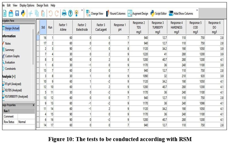 | Figure 10: The tests to be conducted according with RSM
|
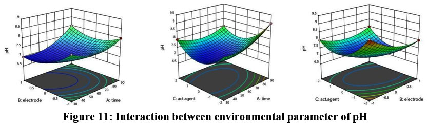
pH
The predicted R2 of 0.9978 matches the adjusted R2 of 0.9997 within a margin of less than 0.2. Figure 11 illustrates the relationship between environmental parameters and pH.
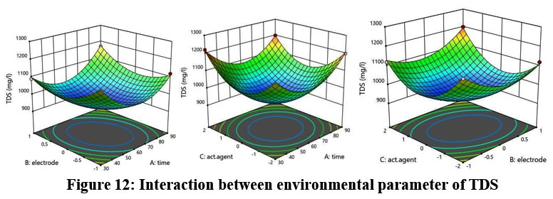
TDS
A difference of less than 0.2 separates the predicted R2 value of 0.9514 from the adjusted R2 value of 0.9997. Figure 12 shows the connection between environmental parameters and TDS.
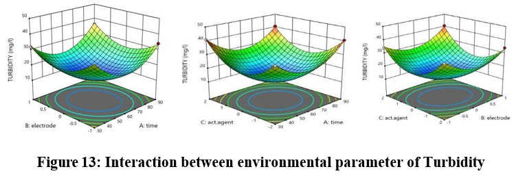
Turbidity
The predicted R2 value of 0.9514 shows acceptable correlation when compared against the adjusted R2 value of 0.9931.Figure 13 illustrates the relationship of environmental variables with Turbidity since the difference remains below 0.2.
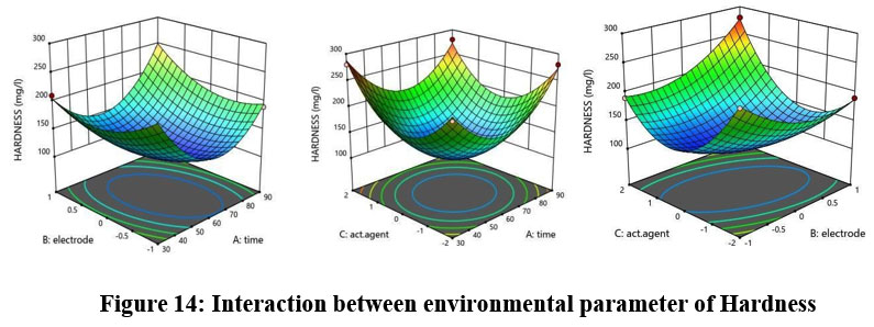
Hardness
The model predicts an R2 value of 0.8903 which stays within reasonable limits compared to the adjusted R2 value of 0.9843. However, the predicted values remains below 0.2 , as figure 14 illustrates the interaction of environmental factors with Hardness measurements.
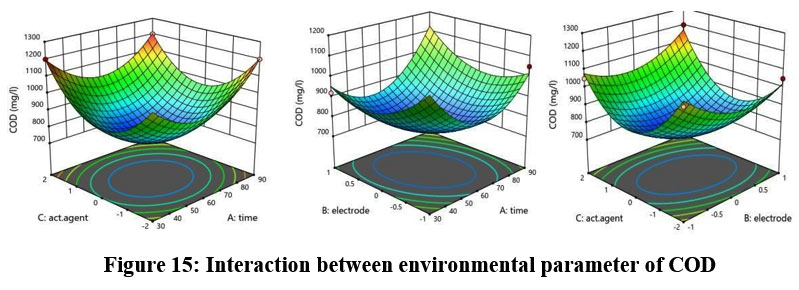
COD
The predicted R2 of 0.7919 exhibits a compatible relationship with the adjusted R2 value of 0.9703 which constitutes a difference of less than 0.2. Figure 15 shows a depiction of the environmental parameter-CPM interaction.
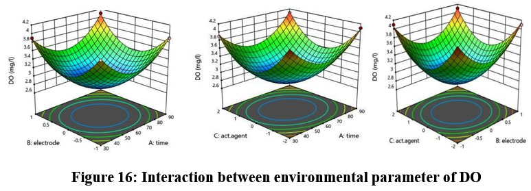
DO
The predicted R2 of 0.9708 shows as match with the adjusted R2 of 0.9958. Figure 16 illustrates DO variation according to environmental parameters and the differences remain less than 0.2.
 | Figure 11: Interaction between environmental parameter of pH
|
 |
|
 | Figure 13: Interaction between environmental parameter of Turbidity
|
 | Figure 14: Interaction between environmental parameter of Hardness
|
 | Figure 15: Interaction between environmental parameter of COD
|
 |
|
Coefficient of R2, in this study shows that the values reached nearly 1 that interprets better fit that shows excellent variability in response. The table 5 shows the significance about the tests and estimate quadratic model parameters, detect lack of fit and to build sequential designs and Table 6 depicts the Fit Statistics of the variability in response.
Table 5: ANOVA result and adequacy of the quadratic model
pH | source | Sum of squares | df | Mean squares | F-value | P-value | |
model | 0.225 | 9 | 0.025 | 5696.5 | <0.0001 | significant | |
A-time | 0.015 | 1 | 0.015 | 3562.9 | <0.0001 | - | |
C-act.agent | 0.01 | 1 | 0.014 | 3343.1 | <0.0001 | - | |
AB | 0.0083 | 1 | 0.0083 | 1894.89 | < 0.0001 | - | |
AC | 0.0074 | 1 | 0.0074 | 1671.55 | < 0.0001 | - | |
BC | 0.0074 | 1 | 0.0074 | 1671.55 | < 0.0001 | - | |
A2 | 0.0198 | 1 | 0.0198 | 4487.90 | < 0.0001 | - | |
B2 | 0.0198 | 1 | 0.0198 | 4487.90 | < 0.0001 | - | |
C2 | 0.1039 | 1 | 0.1039 | 23592.8 | < 0.0001 | - | |
Residual | 0.000 | 7 | 4.403 | - | - | - | |
Lack of fit | 0.000 | 3 | 0.0000 | - | - | - | |
Pure error | 0.000 | 4 | 0.0000 | - | - | - | |
Cor total | 0.2258 | 16 | - | - | - | - | |
TURBIDITY | model | 2153.92 | 9 | 239.32 | 255.08 | <0.0001 | significant |
A-time | 5.44 | 1 | 5.44 | 5.80 | 0.0468 | - | |
B-electrode | 0.7812 | 1 | 0.7812 | 0.8327 | 0.3918 | - | |
C-act.agent | 11.76 | 1 | 11.76 | 12.54 | 0.0095 | - | |
AB | 8.41 | 1 | 8.41 | 8.96 | 0.0201 | - | |
AC | 6.25 | 1 | 6.25 | 6.66 | 0.0364 | - | |
BC | 17.22 | 1 | 17.22 | 18.36 | 0.0036 | -- | |
A2 | 667.14 | 1 | 667.14 | 711.07 | <0.0001 | - | |
B2 | 361.24 | 1 | 361.24 | 385.03 | <0.0001 | - | |
C2 | 862.52 | 1 | 862.52 | 919.32 | <0.0001 | - | |
Residual | 6.57 | 7 | 0.9382 | - | - | - | |
Lack of fit | 6.57 | 3 | 2.19 | - | - | - | |
Pure error | 0.0000 | 4 | 0.0000 | - | - | - | |
Cor total | - | - | - | - | - | - | |
HARDNESS | Model | 72394.12 | 9 | 8043.79 | 112.61 | <0.0001 | significant |
A-time | 50.00 | 1 | 50.00 | 0.7000 | 0.4304 | - | |
B-electrode | 450.00 | 1 | 450.00 | 6.30 | 0.0404 | -- | |
C-act.agent | 800.00 | 1 | 800.00 | 11.20 | 0.0123 | - | |
AB | 1600.00 | 1 | 1600.00 | 22.40 | 0.0021 | - | |
AC | 400.00 | 1 | 400.00 | 5.60 | 0.0499 | - | |
BC | 4900.00 | 1 | 4900.00 | 68.60 | <0.0001 | - | |
A² | 25289.47 | 1 | 25289.47 | 354.05 | <0.0001 | - | |
B² | 4447.37 | 1 | 4447.37 | 62.26 | <0.0001 | - | |
C² | 28657.89 | 1 | 28657.89 | 401.21 | <0.0001 | - | |
Residual | 500.00 | 7 | 71.43 | - | - | - | |
Lack of Fit | 500.00 | 3 | 166.67 | - | - | - | |
Pure Error | 0.0000 | 4 | 0.0000 | - | - | - | |
Cor Total | 72894.12 | 16 | - | - | - | - | |
COD | Model | 5.191 | 9 | 57682.66 | 59.02 | <0.0001 | significant |
A-time | 6612.50 | 1 | 6612.50 | 6.77 | 0.0354 | - | |
B-electrode | 98.00 | 1 | 98.00 | 0.1003 | 0.7607 | - | |
C-act.agent | 5100.50 | 1 | 5100.50 | 5.22 | 0.0563 | - | |
AB | 13225.00 | 1 | 13225.00 | 13.53 | 0.0079 | - | |
AC | 2500.00 | 1 | 2500.00 | 2.56 | 0.1538 | - | |
BC | 9801.00 | 1 | 9801.00 | 10.03 | 0.0158 | - | |
A² | 1.426E+05 | 1 | 1.426E+0 | 145.86 | <0.0001 | - | |
B² | 49567.37 | 1 | 49567.37 | 50.72 | 0.0002 | - | |
C² | 2.446E+05 | 1 | 2.446E+0 | 250.24 | <0.0001 | - | |
Residual | 6841.00 | 7 | 977.29 | - | - | - | |
Lack of Fit | 6841.00 | 3 | 2280.33 | - | - | - | |
Pure Error | 0.0000 | 4 | 0.0000 | - | - | - | |
Cor Total | 5.260 | 16 | - | - | - | - | |
DO | Model | 5.47 | 9 | 0.6073 | 425.08 | <0.0001 | significant |
A-time | 0.0200 | 1 | 0.0200 | 14.00 | 0.0072 | - | |
B-electrode | 0.0050 | 1 | 0.0050 | 3.50 | 0.1036 | - | |
C-act.agent | 0.0050 | 1 | 0.0050 | 3.50 | 0.1036 | - | |
AB | 0.0100 | 1 | 0.0100 | 7.00 | 0.0331 | - | |
AC | 0.0100 | 1 | 0.0100 | 7.00 | 0.0331 | - | |
BC | 0.0000 | 1 | 0.0000 | 0.0000 | 1.0000 | - | |
A² | 1.27 | 1 | 1.27 | 891.58 | <0.0001 | - | |
B² | 1.52 | 1 | 1.52 | 1061.05 | <0.0001 | - | |
C² | 2.06 | 1 | 2.06 | 1444.21 | <0.0001 | - | |
Residual | 0.0100 | 7 | 0.0014 | - | - | - | |
Lack of Fit | 0.0100 | 3 | 0.0033 | - | - | - | |
Pure Error | 0.0000 | 4 | 0.0000 | - | - | - | |
Cor Total | 5.48 | 16 | - | - | - | - | |
TDS | Model | 1.926E+05 | 9 | 21400.33 | 272.37 | < 0.0001 | significant |
A-time | 200.00 | 1 | 200.00 | 2.55 | 0.1546 | - | |
B-electrode | 0.0000 | 1 | 0.0000 | 0.0000 | 1.0000 | - | |
C-act.agent | 800.00 | 1 | 800.00 | 10.18 | 0.0153 | - | |
AB | 4225.00 | 1 | 4225.00 | 53.77 | 0.0002 | - | |
AC | 625.00 | 1 | 625.00 | 7.95 | 0.0258 | - | |
BC | 4225.00 | 1 | 4225.00 | 53.77 | 0.0002 | - | |
A² | 61901.32 | 1 | 61901.32 | 787.83 | < 0.0001 | - | |
B² | 24480.26 | 1 | 24480.26 | 311.57 | < 0.0001 | - | |
C² | 78164.47 | 1 | 78164.47 | 994.82 | < 0.0001 | - | |
Residual | 550.00 | 7 | 78.57 | - | - | - | |
Lack of Fit | 550.00 | 3 | 183.33 | - | - | - | |
Pure Error | 0.0000 | 4 | 0.0000 | - | - | - | |
Cor Total | 1.93 | 16 | - | - | - | - |
Table 6: Fit Statistics
pH | Std.dev | 0.0021 | R2 | 0.9999 |
mean | 2.78 | Adjusted R2 | 0.9997 | |
C.V% | 0.0574 | Predicted R2 | 0.9978 | |
1 | Adeq Precision | 220.9897 | ||
TDS | Std.dev | 0.9686 | R2 | 0.9970 |
mean | 29.72 | Adjusted R2 | 0.9931 | |
C.V% | 3.26 | Predicted R2 | 0.9514 | |
Adeq Precision | 38.4140 | |||
TURBIDITY | Std.dev | 0.9686 | R2 | 0.9970 |
mean | 29.72 | Adjusted R2 | 0.9931 | |
C.V% | 3.26 | Predicted R2 | 0.9514 | |
Adeq Precision | 38.4140 | |||
HARDNESS | Std.dev | 8.45 | R2 | 0.9931 |
mean | 200.59 | Adjusted R2 | 0.9843 | |
C.V% | 4.21 | Predicted R2 | 0.8903 | |
Adeq Precision | 27.3834 | |||
COD | Std.dev | 31.26 | R2 | 0.9870 |
mean | 1001.06 | AdjustedR2 | 0.9703 | |
C.V% | 3.12 | Predicted R2 | 0.7919 | |
Adeq Precision | 18.9352 | |||
DO | Std.dev | 0.0378 | R2 | 0.9982 |
mean | 3.676 | Adjusted R2 | 0.9958 | |
C.V% | 1.03 | Predicted R2 | 0.9708 | |
Adeq Precision | 46.5701 |
The confirmation point is adhered as 60,0,0 which indicates calcium carbonate adsorbent works good in grey water improvement with copper electrode at 60 minutes.
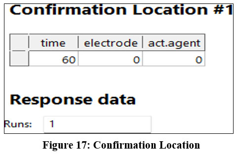 | Figure 17: Confirmation Location
|
Discussion
The procured results is observed that the optimum condition for electro- coagulation of grey water is at 60 minutes with calcium carbonate activated banana bract by using copper electrode, and can be concluded by an efficiency strategy of runs where on this particular conditions the pH, TDS, Turbidity, Hardness, COD, DO as 84%,85%,74%,75%,85%,80% and the total efficiency is attained as 82% is attained in improving grey water.
Conclusion
The Electro coagulation is simple treatment process using aluminum, copper and stainless-steel electrodes with different adsorbents. The effect of process was examined in removal of pH, TDS, Turbidity, COD, etc. Results showed that optimum removal of contaminants are achieved at 60 minutes by Cu-Cu electrode with CaCo3 as adsorbent with a total efficiency of 82%. A 3D surface plot constructed by RSM shows the optimal confirmation points that require minimal testing runs. The analysis shows the developed quadratic model successfully matches experimental data through 95% assessment of variance model optimization. The future studies may be conducted to analyze the wetland cultivation viability on plant growth and yield or can be used to recharge ground water. This study indicates that grey effluent is let into environment without affecting the quality of nature and can be utilized as a revival resource in replenishing the riverine areas and can be used as industrial coolants.
Acknowledgement
I would like to thank all the staff members of the Department of Environmental engineering, Government College of Technology Coimbatore, for their help and encouragement.
Funding Sources
The author(s) received no financial support for the research, authorship, and/or publication of this article.
Conflicts of Interest
The authors do not have any conflict of interest
Data Availability Statement
The manuscript incorporates all datasets produced or examined throughout this research study.
Ethics Statement
This research did not involve human participants, animal subjects, or any material that requires ethical approval.
Informed Consent Statement
This study did not involve human participants, and therefore, informed consent was not required.
Permission to Reproduce Material from Other Sources
Not Applicable
Author Contributions
Charlotte Mashiya Rajesh- Conceived methodology and writing original draft.
Ravathi Mohanadas Chandrika- Data collection and manuscript critical revision
Revathi- Contributed in data analysis
References
- Pushparaj Patel, Shubhi Gupta andet al., Electrocoagulation process for greywater treatment: statistical modeling, optimization, cost analysis and sludge management. Separation and purification technology.2022;296(1): 121327.
CrossRef - Musfque Ahmed, Meenakshi Arora. Suitability of grey water recycling as decentralized alternative water supply option for integrated urban water management. IOSR journal of Engineering.2012;2(9):31-35
CrossRef - Eriksson E, Srigirishetty S and et al.Organic matter and heavy metal in grey water sludge. International Journal of Water SA.2020, 36(1): 139-142.
CrossRef - Sergi Garcia-Segura, Maria Maesia S.G. Eiband. Electrocoagulation and advanced electrocoagulation processes: A general review about the fundamentals, emerging applications and its association with other technologies.2017; 801:267- 299
CrossRef - Snehal Joshi, Priti Palande and et al.,this “ Purification of Grey water using the natural method”. International Journal of Environment, Agriculture and Biotechnology.2022, 7(2).
CrossRef - O. Cherkas, T. Beuvier, S. Fall, A. Gibaud. "X-ray absorption and diffraction analysis for determination of the amount of calcium carbonate and porosity in paper sheets", Cellulose, 2016
CrossRef - Bazrafshan E, Moein H, Kord Mostafapour F, Nakhaie S. Application of Electrocoagulation Process for Dairy Wastewater Treatment. Journal of Chemistry. 2013;77(1): 117-124.
CrossRef - Ravikumar Konda Venkata Giri, Liji Susan Raju, Yarlagadda Venkata Nancharaiah, Mrudula Pulimi et al. "Anaerobic nano zero-valent iron granules for hexavalent chromium removal from aqueous solution", Environmental Technology & Innovation, 2019
- Zhang Yingjie, Zhao Shuying, Tang Zhimin, Li Yan, Wang Lu. "Layer-by-layer assembly of peptides,decorated coaxial nanofibrous membranes with antibiofilm and visual pH sensing capability", Colloids and Surfaces B: Biointerfaces, 2022.
CrossRef


